Multiclass Diffential Expression Analysis
Multi-class / Multi-group Differential Expression Analysis
Introduction
In transcriptomics analysis, we are often interested in identifying differentially expressed genes. For example, if we have two conditions or cell types, we may be interested in what genes are significantly upregulated in condition A vs. B or cell type X vs. Y and vice versa. However, what happens when you have multiple conditions or many cell types? In this tutorial, I will use simulated data to demonstrate potential stategies for performing multi-class or multi-group differential expression analysis.
Simulation
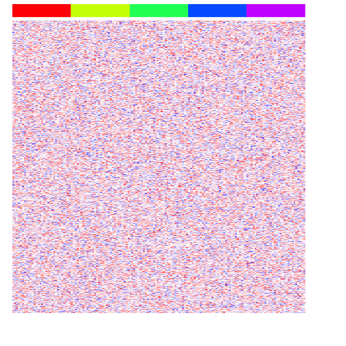
First, let’s simulate 5 different classes/groups of samples (say, bulk RNA-seq of 5 different sorted cell types), each with 30 samples each, each expressing 1000 genes total. Note, in this very simplistic demonstration, we will assume that our gene expression follow a normal distribution.
set.seed(0)
G <- 5
N <- 30
M <- 1000
initmean <- 5
initvar <- 10
mat <- matrix(rnorm(N*M*G, initmean, initvar), M, N*G)
rownames(mat) <- paste0('gene', 1:M)
colnames(mat) <- paste0('cell', 1:(N*G))
group <- factor(sapply(1:G, function(x) rep(paste0('group', x), N)))
names(group) <- colnames(mat)
heatmap(mat, Rowv=NA, Colv=NA, col=colorRampPalette(c('blue', 'white', 'red'))(100), scale="none", ColSideColors=rainbow(G)[group], labCol=FALSE, labRow=FALSE)
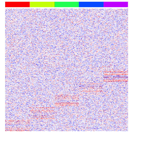
Now, let’s simulate some differentially upregulated genes unique to each group.
set.seed(0)
upreg <- 5
upregvar <- 10
ng <- 100

diff <- lapply(1:G, function(x) {
  diff <- rownames(mat)[(((x-1)*ng)+1):(((x-1)*ng)+ng)]
  mat[diff, group==paste0('group', x)] <<- mat[diff, group==paste0('group', x)] + rnorm(ng, upreg, upregvar)
  return(diff)
})
names(diff) <- paste0('group', 1:G)

heatmap(mat, Rowv=NA, Colv=NA, col=colorRampPalette(c('blue', 'white', 'red'))(100), scale="none", ColSideColors=rainbow(G)[group], labCol=FALSE, labRow=FALSE)
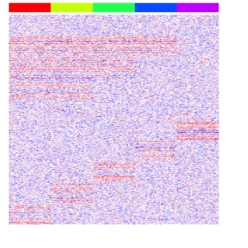
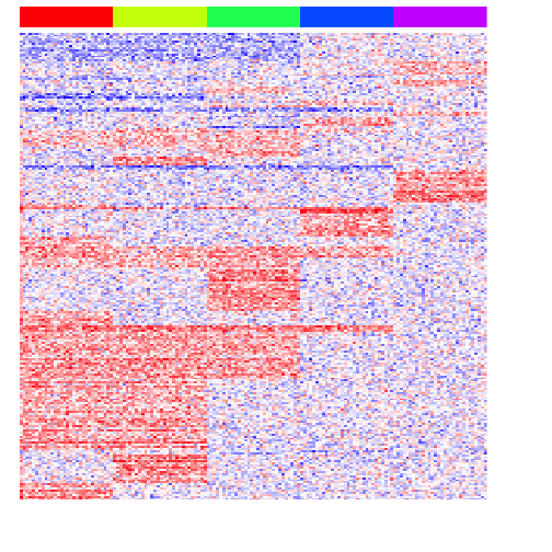
Let’s also simulate some differentially upregulated genes affecting groups of groups. This is typical of cell differentiation processes.
diff2 <- lapply(2:(G-1), function(x) {
  y <- x+G
  diff <- rownames(mat)[(((y-1)*ng)+1):(((y-1)*ng)+ng)]
  mat[diff, group %in% paste0("group", 1:x)] <<- mat[diff, group %in% paste0("group", 1:x)] + rnorm(ng, upreg, upregvar)
  return(diff)
})

heatmap(mat, Rowv=NA, Colv=NA, col=colorRampPalette(c('blue', 'white', 'red'))(100), scale="none", ColSideColors=rainbow(G)[group], labCol=FALSE, labRow=FALSE)
Now, we can begin testing different approaches for multi-group differential expression analysis.
1 vs many (in group vs. not in group)
One approach is to consider each group vs. all others. We can use a simple T-test to test whether each gene is significantly upregulated in each group vs. all other groups.
pv.sig <- lapply(levels(group), function(g){
ingroup <- names(group)[group %in% g]
outgroup <- names(group)[!(group %in% g)]
pv <- sapply(1:M, function(i) {
t.test(mat[i,ingroup], mat[i,outgroup], alternative='greater')$p.value
#t.test(mat[i,ingroup], mat[i,outgroup])$p.value
})
names(pv) <- rownames(mat)
pv.sig <- names(pv)[pv < 0.05/M/G] ## bonferonni
pv.sig
})
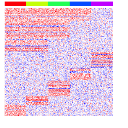
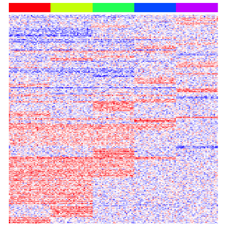
heatmap(mat[unique(unlist(pv.sig)),], Rowv=NA, Colv=NA, col=colorRampPalette(c('blue', 'white', 'red'))(100), scale="none", ColSideColors=rainbow(G)[group], labCol=FALSE, labRow=FALSE)

Indeed, we pick up many of the differentially upregulated genes we simulated that are unique to each group ie. in diff. However, we have a much harder time picking up the differentially upregulated genes marking multiple groups, ie. in diff2 as expected.
perf <- function(pv.sig) {
  predtrue <- unique(unlist(pv.sig)) ## predicted differentially expressed genes
  predfalse <- setdiff(rownames(mat), predtrue) ## predicted not differentially expressed genes
  true <- c(unlist(diff), unlist(diff2)) ## true differentially expressed genes
  false <- setdiff(rownames(mat), true) ## true not differentially expressed genes
  TP <- sum(predtrue %in% true)
  TN <- sum(predfalse %in% false)
  FP <- sum(predtrue %in% false)
  FN <- sum(predfalse %in% true)
  sens <- TP/(TP+FN)
  spec <- TN/(TN+FP)
  prec <- TP/(TP+FP)
  fdr <- FP/(TP+FP)
  acc <- (TP+TN)/(TP+FP+FN+TN)
  return(data.frame(sens, spec, prec, fdr, acc))
}
print(perf(pv.sig))
##      sens spec prec fdr   acc
## 1 0.25625    1    1   0 0.405
ANOVA
Alternatively, we can use ANOVA (analysis of variance) to identify genes that are variable among and between groups.
pv <- sapply(1:M, function(i) {
  mydataframe <- data.frame(y=mat[i,], ig=group)
  fit <- aov(y ~ ig, data=mydataframe)
  summary(fit)[[1]][["Pr(>F)"]][1]
})
names(pv) <- rownames(mat)
pv.sig <- names(pv)[pv < 0.05/M/G] ## bonferonni

heatmap(mat[pv.sig,], Rowv=NA, Colv=NA, col=colorRampPalette(c('blue', 'white', 'red'))(100), scale="none", ColSideColors=rainbow(G)[group], labCol=FALSE, labRow=FALSE)
Note with ANOVA, we need to do an additional step to then figure out which group the variable gene is marking. But compared to testing each group vs. all others, we do get more genes that are differentially upregulated in multiple groups.
print(perf(pv.sig))
##     sens spec prec fdr  acc
## 1 0.3625    1    1   0 0.49
Testing combined groups (pairs, triplets, etc)
What if we test all possible pairwise combinations of groups?
pv.sig.pair <- lapply(levels(group), function(g1) {
  g2 <- setdiff(levels(group), g1)
  unlist(lapply(g2, function(g) {
    ## test two groups vs. all others
    ingroup <- names(group)[group %in% c(g1, g)]
    outgroup <- names(group)[!(group %in% c(g1, g))]
    pv <- sapply(1:M, function(i) {
      t.test(mat[i,ingroup], mat[i,outgroup], alternative='greater')$p.value
    })
    names(pv) <- rownames(mat)
    pv.sig <- names(pv)[pv < 0.05/M/G] ## bonferonni
    pv.sig
  }))
})

heatmap(mat[unique(unlist(pv.sig.pair)),], Rowv=NA, Colv=NA, col=colorRampPalette(c('blue', 'white', 'red'))(100), scale="none", ColSideColors=rainbow(G)[group], labCol=FALSE, labRow=FALSE)
As expected, we now readily recover the genes upregulated in two groups.
print(perf(pv.sig.pair))
##      sens spec prec fdr   acc
## 1 0.28125    1    1   0 0.425
Of course, this approach becomes unreasonable if we have many groups. And if we are doing all pairs, why not all triplets. The number of combinations grow exponentially and quickly becomes intractable.
pv.sig.trip <- lapply(levels(group), function(g1) {
  g2 <- setdiff(levels(group), g1)
  unlist(lapply(g2, function(gi) {
    g3 <- setdiff(levels(group), gi)
    unlist(lapply(g3, function(gj) {
      ## test three groups vs. all others
      ingroup <- names(group)[group %in% c(g1, gi, gj)]
      outgroup <- names(group)[!(group %in% c(g1, gi, gj))]
      pv <- sapply(1:M, function(i) {
        t.test(mat[i,ingroup], mat[i,outgroup], alternative='greater')$p.value
      })
      names(pv) <- rownames(mat)
      pv.sig <- names(pv)[pv < 0.05/M/G] ## bonferonni
      pv.sig
    }))
  }))
})

heatmap(mat[unique(unlist(pv.sig.trip)),], Rowv=NA, Colv=NA, col=colorRampPalette(c('blue', 'white', 'red'))(100), scale="none", ColSideColors=rainbow(G)[group], labCol=FALSE, labRow=FALSE)
print(perf(pv.sig.trip))
##      sens  spec      prec         fdr  acc
## 1 0.32625 0.995 0.9961832 0.003816794 0.46
Tree-based binary split
My preferred approach is to assume an underlying tree structure relating groups and compare groups based on recursive binary splits along the tree.
## average gene expression for each group
mat.group <- do.call(cbind, lapply(levels(group), function(g) {
rowMeans(mat[,group==g])
}))
colnames(mat.group) <- levels(group)
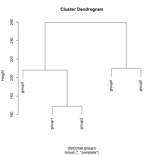
## construct tree related groups
hc <- hclust(dist(t(mat.group)), method='complete')
plot(hc)
dend <- as.dendrogram(hc)
pv.sig.all <- c()

pv.recur <- function(dend) {
  g1 <- labels(dend[[1]])
  g2 <- labels(dend[[2]])
  #print(g1)
  #print(g2)
  ingroup <- names(group)[group %in% g1]
  outgroup <- names(group)[group %in% g2]
  pv <- sapply(1:M, function(i) {
      t.test(mat[i,ingroup], mat[i,outgroup])$p.value
  })
  names(pv) <- rownames(mat)
  pv.sig <- names(pv)[pv < 0.05/M/length(hc$height)] ## bonferonni
  #print(pv.sig)
  pv.sig.all <<- c(pv.sig.all, pv.sig) ## save

  ## recursion to go down tree if not leaf
  if(!is.leaf(dend[[1]])) {
    pv.recur(dend[[1]])
  }
  if(!is.leaf(dend[[2]])) {
    pv.recur(dend[[2]])
  }
}
pv.recur(dend)

heatmap(mat[unique(unlist(pv.sig.all)),], Rowv=NA, Colv=NA, col=colorRampPalette(c('blue', 'white', 'red'))(100), scale="none", ColSideColors=rainbow(G)[group], labCol=FALSE, labRow=FALSE)
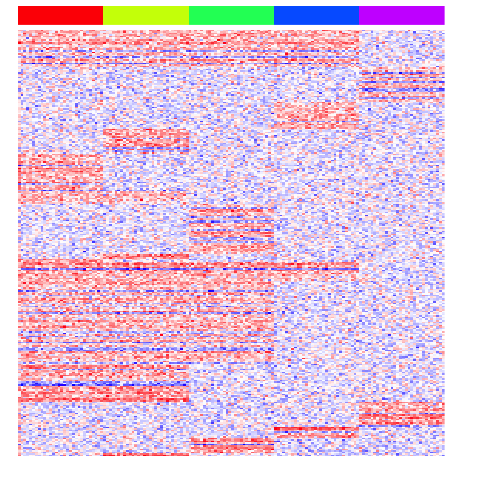
Of course, the performance of this approach will depend on the initial tree reconstruction.
print(perf(pv.sig.all))
##   sens spec prec fdr   acc
## 1 0.34    1    1   0 0.472
Conclusion
Try it yourself! What happens if we reduce the degree of upregulation upreg in the simulation? Or increase in variance? What if instead of using a normal, we simulate a zero-inflated negative binomial more characteristic of single cell RNA-seq data? What if we add in different levels of noise to each sample, differential library sizes, and so forth?
Recent Posts
- AI-guided data visualization of gas prices in different geographical locations across the US over time on 04 May 2026
- The Mentorship Index on 01 March 2026
- Vibe coding with SEraster and STcompare to compare spatial transcriptomics technologies on 22 February 2026
- RNA velocity in situ infers gene expression dynamics using spatial transcriptomics data on 13 October 2025
- Analyzing ICE Arrest Data - Part 2 on 27 September 2025