HW5: Multi-Panel Data Visualization of the White Pulp Tissue Structure in the CODEX Data

I am an undergraduate student majoring in Biomedical Engineering at Johns Hopkins University.

HW5: Multi-Panel Data Visualization of the White Pulp Tissue Structure in the CODEX Data

Perform a full analysis (quality control, dimensionality reduction, kmeans clustering, differential expression analysis) on your data. Your goal is to figure out what tissue structure is represented in the CODEX data. Options include: (1) Artery/Vein, (2) White pulp, (3) Red pulp, (4) Capsule/Trabecula. You will need to visualize and interpret at least two cell-types. Create a data visualization and write a description to convince me that your interpretation is correct.

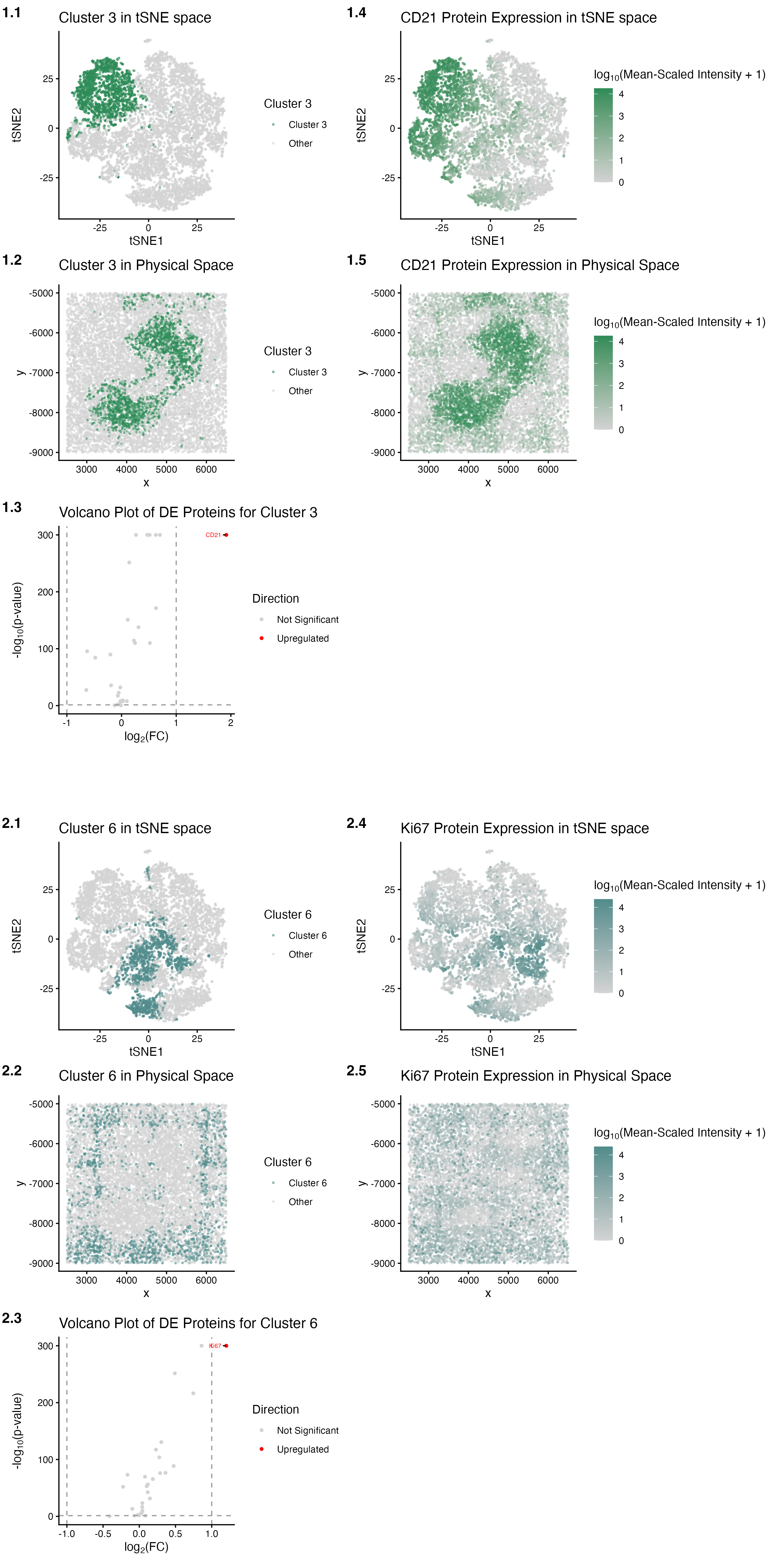
The figures identify Clusters 3 and 6 as coherent and spatially localized clusters of cells in the CODEX data that have distinct protein expressions. K-means clustering was performed using k (centers) = 6, since this optimal k value was at the elbow of the scree plot depicting the total withinness on the y-axis and the number of centroids k on the x-axis. Initial examination of the reduced dimensional space of PCA led to the selection of Clusters 3 and 6 as the clusters of interest, as they not only had minimal overlap with each other, but also with all of the remaining clusters, and were distinctly congregated.

In panel 1.1, Cluster 3 (sea green) was found to form a distinct cluster of cells in the non-linearly reduced dimensional space of tSNE (light grey). In panel 1.2, Cluster 3 (sea green) was found to be concentrated in a spatially localized, compact region, implying the marking of an anatomically organized compartment in the physical space (light grey). In panel 1.3, Cluster 3 shows its differentially expressed proteins that are upregulated (red; i.e., CD21) and not significantly changed in expression (light grey) compared to protein expressions in all of the remaining clusters; no proteins with significantly downregulated expression were detected. Given that CD21 was found to be a differentially upregulated protein in Cluster 3 (pval = 1.000000e-300, log2fc = 1.91645311) through the examination of outputs from the two-sided Wilcoxon rank-sum test performed to depict the volcano plot in panel 1.3, it was selected as a potential marker protein for Cluster 3. In panel 1.4, cells that highly express CD21 (sea green) were found to form a distinct cluster in the non-linearly reduced dimensional space of tSNE (light grey), indicating the CD21 protein’s role as a marker protein for Cluster 3. In panel 1.5, cells that highly express CD21 (sea green) were found to be concentrated in a spatially localized, compact region, implying the marking of an anatomically organized compartment in the physical space (light grey). This compact region is also spatially co-localized to that formed by Cluster 3 in the physical space, further validating the CD21 protein’s role as a marker protein for the proteomically distinct Cluster 3 in the CODEX dataset.

In panel 2.1, Cluster 6 (dark slate gray) was found to form a distinct cluster of cells in the non-linearly reduced dimensional space of tSNE (light grey). In panel 2.2, Cluster 6 (dark slate gray) was found to be concentrated in a spatially enclosing and nested region, implying the marking of an anatomically organized compartment in the physical space (light grey). In panel 2.3, Cluster 6 shows its differentially expressed proteins that are upregulated (red; i.e., Ki67) and not significantly changed in expression (light grey) compared to protein expressions in all of the remaining clusters; no proteins with significantly downregulated expression were detected. Given that Ki67 was found to be a differentially upregulated protein in Cluster 6 (pval = 1.000000e-300, log2fc = 1.201308048) through the examination of outputs from the two-sided Wilcoxon rank-sum test performed to depict the volcano plot in panel 2.3, it was selected as a potential marker protein for Cluster 6. In panel 2.4, cells that highly express Ki67 (dark slate gray) were found to form a distinct cluster in the non-linearly reduced dimensional space of tSNE (light grey), indicating the Ki67 protein’s role as a marker protein for Cluster 6. In panel 2.5, cells that highly express Ki67 (dark slate gray) were found to be concentrated in a spatially enclosing and nested region, implying the marking of an anatomically organized compartment in the physical space (light grey). This nested region is also spatially co-localized to that formed by Cluster 6 in the physical space, further validating the Ki67 protein’s role as a marker protein for the proteomically distinct Cluster 6 in the CODEX dataset.

The tissue structure represented in the CODEX data is the white pulp. The first cell-type visualized and interpreted is speculated to be follicular dendritic cells (FDCs). The CD21 protein marker (encoded by the Cr2/CD21 gene), upregulated in Cluster 3, has been characterized, through staining, to be a defining marker for FDCs that form a moderately dense, diffuse meshwork in the center of the white pulp nodules, fading towards the periphery[1],[2]. The second cell-type visualized and interpreted is speculated to be Ki67+ germinal center B cells (GCBCs). The Ki67 protein marker (encoded by the Mki67 gene), upregulated in Cluster 6, has been characterized, through staining, to be a nuclear protein marker of cellular proliferation that is highly expressed in GCBCs spatially close to FDCs, within the white pulp[2],[3],[4],[5]. Through comparison with the existing literature, my analysis is also spatially validated through the panels 1.5 and 2.5 depicting each of the two marker proteins in the physical space. This is because they exhibit FDCs from Cluster 3, which are stromal cells located in the germinal center, forming a dense network that traps antigen-antibody complexes, which the GCBCs from Cluster 6 interact with for rapid expansion and differentiation[6],[7]. Overall, the anatomical localizations of Clusters 3 and 6 in the human spleen, and references from the literature that discuss the roles of the upregulated proteins in FDCs and GCBCs, found in their respective clusters, strongly support that the tissue structure represented in the CODEX data corresponds to the white pulp of the spleen.

[1] https://doi.org/10.1182/blood.V84.11.3828.bloodjournal84113828

[2] https://doi.org/10.1182/blood-2012-04-424648

[3] https://doi.org/10.1084/jem.20030495

[4] https://doi.org/10.1016/j.celrep.2020.108376

[5] https://doi.org/10.1080/10428199009169601

[6] https://doi.org/10.1016/j.immuni.2016.09.001

[7] https://doi.org/10.1111/j.1365-2567.2004.02075.x

Code

# Load the necessary libraries
library(ggplot2)
library(Rtsne)
library(ggrepel)
library(patchwork)

# Read in data
data <- read.csv('~/Documents/genomic-data-visualization-2026/data/codex_spleen2.csv.gz')
pos <- data[,c('x', 'y')]
rownames(pos) <- data[,1]
pexp <- data[, 4:ncol(data)]
rownames(pexp) <- data[,1]

# Normalize
# Prompt to AI: "Specific ways to normalize the protein expression data in a CODEX dataset using R coding?"
mat <- log10(pexp/rowSums(pexp) * mean(rowSums(pexp))+1)

# PCA: linear dimensionality reduction
pcs <- prcomp(mat, center=TRUE, scale=FALSE)
plot(pcs$sdev[1:50]) # Scree plot: Will perform tSNE on top 9 PCs as it reaches the elbow of the graph

# tSNE: non-linear dimensionality reduction
set.seed(21926)
tsne <- Rtsne::Rtsne(pcs$x[, 1:9], dims=2, perplexity=30, verbose=TRUE)
emb <- tsne$Y
rownames(emb) <- rownames(mat)
colnames(emb) <- c('tSNE1', 'tSNE2')

# Determining the optimal k value for K-means clustering
totw <- sapply(2:25, function(k) {kmeans(pcs$x[,1:9], centers = k, nstart = 10, iter.max = 500, algorithm = "Lloyd")$tot.withinss})
df_totw <- data.frame(k = 2:25, tot.withinss = totw)
ggplot(df_totw, aes(x = k, y = tot.withinss)) + geom_point() + geom_line() + theme_test() # Scree plot: Optimal k = 6 found for K-means clustering

# K-means clustering
clusters <- as.factor(kmeans(pcs$x[,1:9], centers = 6)$cluster)
df_km <- data.frame(pcs$x, clusters)
ggplot(df_km, aes(x=PC1, y=PC2, col=clusters)) + geom_point(size = 0.5) # PC1 vs PC2: Selected clusters 3 and 6 as the one transcriptionally distinct clusters of cells

# Define labels for cluster 3 versus other clusters and cluster 6 versus other clusters
cluster_label_3 <- ifelse(clusters == "3", "Cluster 3", "Other")
cluster_label_6 <- ifelse(clusters == "6", "Cluster 6", "Other")
cluster_3 <- clusters == "3"
cluster_6 <- clusters == "6"
othercells_cluster_3 <- clusters != "3"
othercells_cluster_6 <- clusters != "6"

# Define colors for cluster 3 versus other clusters and cluster 6 versus other clusters
cluster.cols <- c("Other" = "lightgrey", "Cluster 3" = "seagreen4", "Cluster 6" = "darkslategray4")

# 1. Plot panels visualizing clusters 3 and 6, each in reduced dimensional space (tSNE)
df_tsne_cluster_3 <- data.frame(
  emb1 = emb[, 1],
  emb2 = emb[, 2],
  cluster = factor(cluster_label_3, levels = c("Cluster 3", "Other"))
)
p1_1 <- ggplot(df_tsne_cluster_3, aes(x = emb1, y = emb2, color = cluster)) +
  geom_point(size = 0.5, alpha = 0.5) +
  theme_classic() +
  scale_color_manual(values = cluster.cols) +
  labs(title = "Cluster 3 in tSNE space",
       x = "tSNE1", y = "tSNE2", color = "Cluster 3")

df_tsne_cluster_6 <- data.frame(
  emb1 = emb[, 1],
  emb2 = emb[, 2],
  cluster = factor(cluster_label_6, levels = c("Cluster 6", "Other"))
)
p1_2 <- ggplot(df_tsne_cluster_6, aes(x = emb1, y = emb2, color = cluster)) +
  geom_point(size = 0.5, alpha = 0.5) +
  theme_classic() +
  scale_color_manual(values = cluster.cols) +
  labs(title = "Cluster 6 in tSNE space",
       x = "tSNE1", y = "tSNE2", color = "Cluster 6")

# 2. Plot panels visualizing clusters 3 and 6, each in physical space
df_phys_cluster_3 <- data.frame(
  x = pos[, 1],
  y = pos[, 2],
  cluster = factor(cluster_label_3, levels = c("Cluster 3", "Other"))
)
p2_1 <- ggplot(df_phys_cluster_3, aes(x = x, y = y, color = cluster)) +
  geom_point(size = 0.5, alpha = 0.5) +
  theme_classic() +
  scale_color_manual(values = cluster.cols) +
  coord_fixed() +
  labs(title = "Cluster 3 in Physical Space", 
       x = "x", y = "y", color = "Cluster 3")

df_phys_cluster_6 <- data.frame(
  x = pos[, 1],
  y = pos[, 2],
  cluster = factor(cluster_label_6, levels = c("Cluster 6", "Other"))
)
p2_2 <- ggplot(df_phys_cluster_6, aes(x = x, y = y, color = cluster)) +
  geom_point(size = 0.5, alpha = 0.5) +
  theme_classic() +
  scale_color_manual(values = cluster.cols) +
  coord_fixed() +
  labs(title = "Cluster 6 in Physical Space", 
       x = "x", y = "y", color = "Cluster 6")

# Compute Wilcoxon p-values (two-sided for volcano plot) for cluster 3 versus other cells
pv_cluster_3 <- sapply(colnames(mat), function(protein) {
  x1 <- mat[cluster_3, protein]
  x2 <- mat[othercells_cluster_3, protein]
  wilcox.test(x1, x2, alternative = "two.sided")$p.value
})
# Avoid p-values of zeros
pv_cluster_3[pv_cluster_3 == 0] <- 1e-300

# Compute log2 fold-change for cluster 3 versus other cells
logfc_cluster_3 <- sapply(colnames(mat), function(protein) {
  log2((mean(mat[cluster_3, protein]) + 1e-6) / (mean(mat[othercells_cluster_3, protein]) + 1e-6))
})

# 3. Plot a panel (volcano plot) visualizing differentially expressed proteins for cluster 3
de_1 <- data.frame(protein = colnames(mat), pval = pv_cluster_3, neglog10p = -log10(pv_cluster_3), log2fc = logfc_cluster_3)
de_1$status <- "Not Significant"
de_1$status[de_1$pval < 0.05 & de_1$log2fc > 1]  <- "Upregulated"
de_1$status[de_1$pval < 0.05 & de_1$log2fc < -1] <- "Downregulated"
p3_1 <- ggplot(de_1, aes(x = log2fc, y = neglog10p, color = status)) +
  geom_point(size = 1) +
  geom_vline(xintercept = c(-1, 1), linetype = "dashed", color = "grey60") +
  geom_hline(yintercept = -log10(0.05), linetype = "dashed", color = "grey60") +
  scale_color_manual(values = c("Downregulated" = "blue",
                                "Not Significant" = "lightgrey",
                                "Upregulated" = "red")) +
  theme_classic() +
  labs(
    title = "Volcano Plot of DE Proteins for Cluster 3",
    x = expression("log"[2]*"(FC)"), 
    y = expression("-log"[10]*"(p-value)"),
    color = "Direction"
  ) +
  geom_text_repel(
    data = subset(de_1, abs(log2fc) > 1 & neglog10p > 10),
    aes(label = protein),
    size = 2,
    max.overlaps = 20,
    show.legend = FALSE,
    segment.color = "black",
    segment.size = 0.5,
    min.segment.length = 0
  )
# Show top DE proteins: selected CD21 as a DE protein from this output (pval = 1.000000e-300, log2fc = 1.91645311, status = Upregulated)
de_1[order(de_1$pval), ]

# Compute Wilcoxon p-values (two-sided for volcano plot) for cluster 6 versus other cells
pv_cluster_6 <- sapply(colnames(mat), function(protein) {
  x1 <- mat[cluster_6, protein]
  x2 <- mat[othercells_cluster_6, protein]
  wilcox.test(x1, x2, alternative = "two.sided")$p.value
})
# Avoid p-values of zeros
pv_cluster_6[pv_cluster_6 == 0] <- 1e-300

# Compute log2 fold-change for cluster 6 versus other cells
logfc_cluster_6 <- sapply(colnames(mat), function(protein) {
  log2((mean(mat[cluster_6, protein]) + 1e-6) / (mean(mat[othercells_cluster_6, protein]) + 1e-6))
})

# 3. Plot a panel (volcano plot) visualizing differentially expressed proteins for cluster 6
de_2 <- data.frame(protein = colnames(mat), pval = pv_cluster_6, neglog10p = -log10(pv_cluster_6), log2fc = logfc_cluster_6)
de_2$status <- "Not Significant"
de_2$status[de_2$pval < 0.05 & de_2$log2fc > 1]  <- "Upregulated"
de_2$status[de_2$pval < 0.05 & de_2$log2fc < -1] <- "Downregulated"
p3_2 <- ggplot(de_2, aes(x = log2fc, y = neglog10p, color = status)) +
  geom_point(size = 1) +
  geom_vline(xintercept = c(-1, 1), linetype = "dashed", color = "grey60") +
  geom_hline(yintercept = -log10(0.05), linetype = "dashed", color = "grey60") +
  scale_color_manual(values = c("Downregulated" = "blue",
                                "Not Significant" = "lightgrey",
                                "Upregulated" = "red")) +
  theme_classic() +
  labs(
    title = "Volcano Plot of DE Proteins for Cluster 6",
    x = expression("log"[2]*"(FC)"), 
    y = expression("-log"[10]*"(p-value)"),
    color = "Direction"
  ) +
  geom_text_repel(
    data = subset(de_2, abs(log2fc) > 1 & neglog10p > 10),
    aes(label = protein),
    size = 2,
    max.overlaps = 20,
    show.legend = FALSE,
    segment.color = "black",
    segment.size = 0.5,
    min.segment.length = 0
  )
# Show top DE proteins: selected Ki67 as a DE protein from this output (pval = 1.000000e-300, log2fc = 1.201308048, status = Upregulated)
de_2[order(de_2$pval), ]

# 4. Plot panels visualizing the CD21 and Ki67 proteins in reduced dimensional space (tSNE)
df_tsne_CD21 <- data.frame(
  emb1 = emb[, 1],
  emb2 = emb[, 2],
  protein = mat[, 'CD21']
)
p4_1 <- ggplot(df_tsne_CD21, aes(x = emb1, y = emb2, color = protein)) +
  geom_point(size = 0.5, alpha = 0.5) +
  theme_classic() +
  scale_color_gradient(low='lightgrey', high='seagreen4') +
  labs(
    title = "CD21 Protein Expression in tSNE space",
    x = "tSNE1", y = "tSNE2", color = expression("log"[10]*"(Mean-Scaled Intensity + 1)")
  )

df_tsne_Ki67 <- data.frame(
  emb1 = emb[, 1],
  emb2 = emb[, 2],
  protein = mat[, 'Ki67']
)
p4_2 <- ggplot(df_tsne_Ki67, aes(x = emb1, y = emb2, color = protein)) +
  geom_point(size = 0.5, alpha = 0.5) +
  theme_classic() +
  scale_color_gradient(low='lightgrey', high='darkslategray4') +
  labs(
    title = "Ki67 Protein Expression in tSNE space",
    x = "tSNE1", y = "tSNE2", color = expression("log"[10]*"(Mean-Scaled Intensity + 1)")
  )

# 5. Plot panels visualizing the CD21 and Ki67  in physical space
df_phys_CD21 <- data.frame(
  x = pos[, 1],
  y = pos[, 2],
  protein = mat[, 'CD21']
)
p5_1 <- ggplot(df_phys_CD21, aes(x = x, y = y, color = protein)) +
  geom_point(size = 0.5, alpha = 0.5) +
  theme_classic() +
  coord_fixed() +
  scale_color_gradient(low='lightgrey', high='seagreen4') +
  labs(
    title = "CD21 Protein Expression in Physical Space",
    x = "x", y = "y", color = expression("log"[10]*"(Mean-Scaled Intensity + 1)")
  )

df_phys_Ki67 <- data.frame(
  x = pos[, 1],
  y = pos[, 2],
  protein = mat[, 'Ki67']
)
p5_2 <- ggplot(df_phys_Ki67, aes(x = x, y = y, color = protein)) +
  geom_point(size = 0.5, alpha = 0.5) +
  theme_classic() +
  coord_fixed() +
  scale_color_gradient(low='lightgrey', high='darkslategray4') +
  labs(
    title = "Ki67 Protein Expression in Physical Space",
    x = "x", y = "y", color = expression("log"[10]*"(Mean-Scaled Intensity + 1)")
  )

# Plot all panels in one plot using patchwork
p1_1_tag <- p1_1 + labs(tag = "1.1") 
p4_1_tag <- p4_1 + labs(tag = "1.4") 
p2_1_tag <- p2_1 + labs(tag = "1.2") 
p5_1_tag <- p5_1 + labs(tag = "1.5") 
p3_1_tag <- p3_1 + labs(tag = "1.3")
p1_2_tag <- p1_2 + labs(tag = "2.1") 
p4_2_tag <- p4_2 + labs(tag = "2.4") 
p2_2_tag <- p2_2 + labs(tag = "2.2") 
p5_2_tag <- p5_2 + labs(tag = "2.5") 
p3_2_tag <- p3_2 + labs(tag = "2.3")
tag_theme <- theme(
  plot.tag.position = c(0, 1),
  plot.tag = element_text(face = "bold")
)
p1_1_tag <- p1_1_tag + tag_theme
p4_1_tag <- p4_1_tag + tag_theme
p2_1_tag <- p2_1_tag + tag_theme
p5_1_tag <- p5_1_tag + tag_theme
p3_1_tag <- p3_1_tag + tag_theme
p1_2_tag <- p1_2_tag + tag_theme
p4_2_tag <- p4_2_tag + tag_theme
p2_2_tag <- p2_2_tag + tag_theme
p5_2_tag <- p5_2_tag + tag_theme
p3_2_tag <- p3_2_tag + tag_theme
plot.layout <- "
AB
CD
E#
##
FG
HI
J#
"
p_all <- p1_1_tag + p4_1_tag + p2_1_tag + p5_1_tag + p3_1_tag + p1_2_tag + p4_2_tag + p2_2_tag + p5_2_tag + p3_2_tag +
  plot_layout(design = plot.layout, widths = c(1, 1),  heights = c(1,1,1,0.35,1,1,1))
ggsave("hw5_yhodo1.png", p_all, width = 10, height = 20, dpi = 300)

19 Feb 2026

« HW5-Interpreting Spleen Tissue Structure from CODEX Spatial Proteomics Data CODEX Spleen Data: White Pulp »