HW5

I am a BME PhD student, curious about science and eager to learn new things.

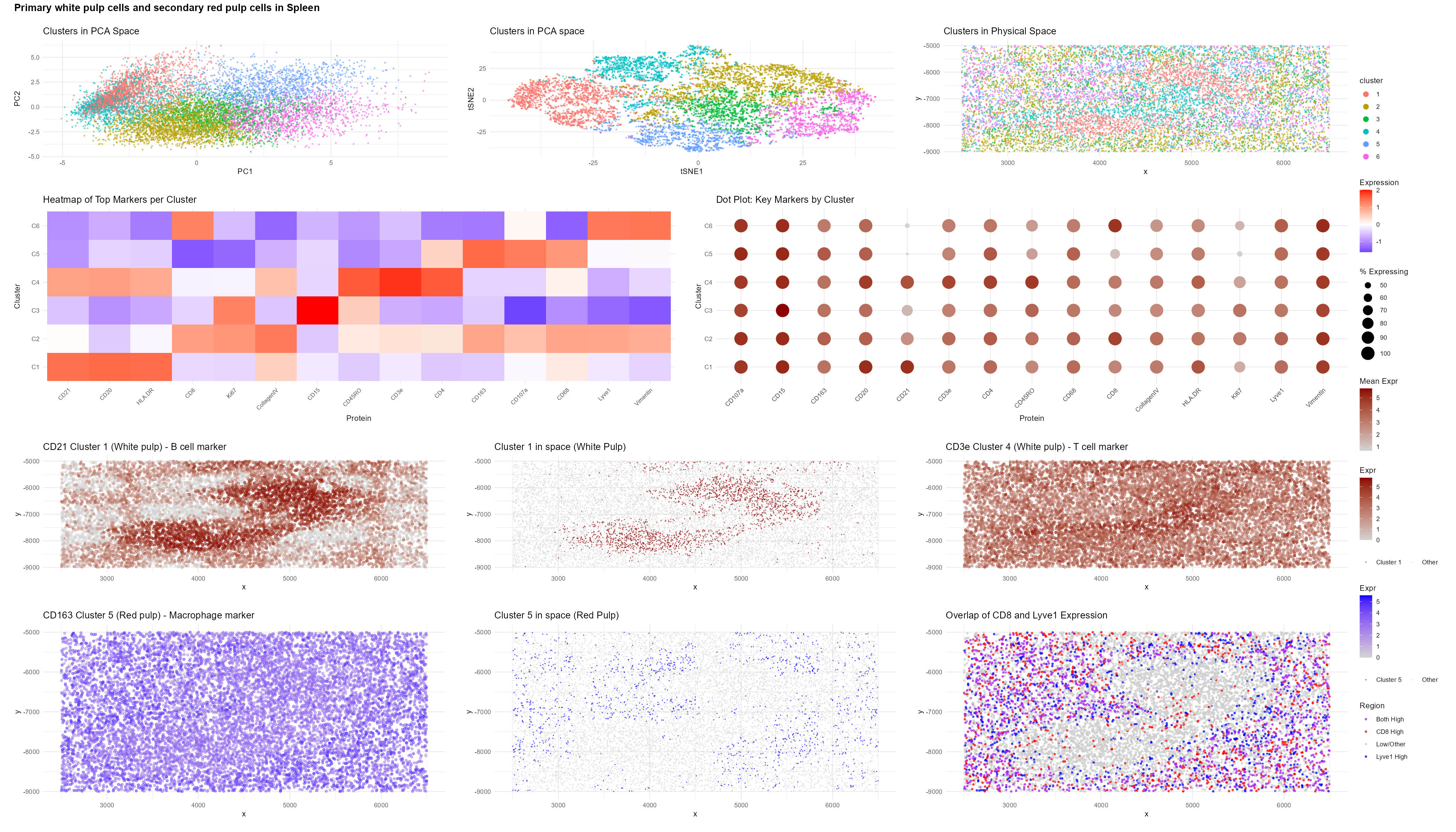
Tissue Structure Identified: White Pulp

Analysis of the CODEX spatial proteomics dataset (codex_spleen2.csv.gz) indicates that the dominant structure in this tissue section is white pulp. The white pulp is the organized lymphoid compartment of the spleen, surrounding central arterioles and consisting primarily of (1) B cell follicles, which support humoral immunity, and (2) the periarteriolar lymphoid sheath (PALS), a T cell–rich zone mediating cell-mediated immune responses (Mebius & Kraal, 2005).

Clustering results, marker enrichment, and spatial organization consistently support this identification.

Cell Types Identified

Cell Type 1: B Cells (Cluster 1)

Cluster 1 showed strong upregulation of CD21 (log2FC = 3.02, padj ≈ 0), CD20 (log2FC = 1.21, padj ≈ 0), and HLA-DR (log2FC = 0.97, padj ≈ 0).

CD20 is a canonical B cell marker (Tedder & Engel, 1994). CD21 supports B cell activation and germinal center formation within splenic follicles (Carroll & Isenman, 2012). HLA-DR enables antigen presentation, a defining feature of B cell function.

Spatially, Cluster 1 formed compact, rounded aggregates consistent with B cell follicles in white pulp. The transcriptional signature and spatial architecture align clearly with follicular B cells.

Cell Type 2: T Cells (Cluster 4)

Cluster 4 was characterized by elevated CD45RO (log2FC = 1.93, padj ≈ 0), CD3e (log2FC = 1.35, padj ≈ 0), and CD4 (log2FC = 0.96, padj ≈ 0).

CD3e is a definitive pan-T cell marker (Clevers et al., 1988). CD4 identifies helper T cells, and CD45RO marks activated or memory T cells.

These cells localized adjacent to and partially surrounding the B cell clusters — a pattern consistent with the PALS region of white pulp, where T cell zones flank B cell follicles (Mebius & Kraal, 2005).

Supporting Evidence: Red Pulp Contrast

Cluster 5 expressed CD163 (log2FC = 0.57, padj = 3.9e-131) and CD68 (log2FC = 0.32, padj = 7.1e-71), markers of tissue-resident macrophages.

CD163 identifies red pulp macrophages responsible for hemoglobin scavenging and erythrocyte clearance (Kristiansen et al., 2001; Nagelkerke et al., 2018). These cells localized outside the lymphoid aggregates, forming a surrounding compartment consistent with red pulp.

The spatial separation between macrophage-rich regions and B/T cell clusters reinforces the identification of white pulp as the central structure in this dataset.

Spatial Delineation by CD8 and Lyve1

Expression patterns of CD8 and Lyve1 further delineated splenic compartments:

High CD8 and low Lyve1 marked organized T cell zones within white pulp.

High Lyve1 marked the sinusoidal network characteristic of red pulp.

This reciprocal spatial pattern clearly distinguishes immune cell clusters from the surrounding vascular filtration compartment.

Analysis Pipeline

The dataset contained 28 protein markers measured across segmented spleen cells. After normalization and log10 transformation, I performed PCA (10 PCs capturing ~80% variance), followed by tSNE (perplexity = 30) for visualization. K-means clustering (K = 6, selected using the elbow method) identified distinct cell populations. Differential expression was assessed using Wilcoxon rank-sum tests with Benjamini–Hochberg correction.

Cluster assignments, spatial localization, and marker expression patterns together support the conclusion that the analyzed region represents splenic white pulp intersparsed with red pulp cells.

References

Mebius, R. E., & Kraal, G. (2005). Structure and function of the spleen. Nature Reviews Immunology, 5(8), 606–616. https://doi.org/10.1038/nri1669
Tedder, T. F., & Engel, P. (1994). CD20: a regulator of cell-cycle progression of B lymphocytes. Immunology Today, 15(9), 450–454. https://doi.org/10.1016/0167-5699(94)90276-3
Carroll, M. C., & Isenman, D. E. (2012). Regulation of humoral immunity by complement. Immunity, 37(2), 199–207. https://doi.org/10.1016/j.immuni.2012.08.002
Clevers, H., Alarcon, B., Wileman, T., & Terhorst, C. (1988). The T cell receptor/CD3 complex: a dynamic protein ensemble. Annual Review of Immunology, 6, 629–662.
Kristiansen, M., Graversen, J. H., Jacobsen, C., et al. (2001). Identification of the haemoglobin scavenger receptor. Nature, 409(6817), 198–201. https://doi.org/10.1038/35051594
Nagelkerke SQ, Bruggeman CW, den Haan JMM, Mul EPJ, van den Berg TK, van Bruggen R, Kuijpers TW. Red pulp macrophages in the human spleen are a distinct cell population with a unique expression of Fc-γ receptors. Blood Adv. 2018 Apr 24;2(8):941-953. doi: 10.1182/bloodadvances.2017015008. PMID: 29692344; PMCID: PMC5916003.
https://www.assaygenie.com/cd-markers-list?srsltid=AfmBOortyzhJgx1eAET28vzn9Nvh5wMj-0gwtKL4xaBxv_uwDUmbGc4V
https://www.labome.com/method/T-Cell-Markers-and-B-Cell-Markers.html
https://www.biorxiv.org/content/10.1101/2021.10.20.465151v2.full.pdf

Code

setwd("C:/Users/John-Paul/Downloads")
data <- read.csv(gzfile("codex_spleen2.csv.gz"))
head(data)

dim(data)
pos <- data[, 2:3]
# Plot x and y positions of the cells
plot(pos)

pexp <- data[, 5:ncol(data)]
rownames(pos) <- rownames(pexp) <- data[, 1]
area <- data[, 4]
names(area) <- data[, 1]

dim(pexp)
colnames(pexp)
head(area)

# Normalize
totpexp <- rowSums(pexp)
mat <- log10(pexp/totpexp * 1e6 + 1)

# Distribution
hist(totpexp, main = "Total Protein Expression", xlab = "Total Expression", breaks = 50)
hist(area, main = "Cell Area", xlab = "Area", breaks = 50)
hist(log10(totpexp + 1), main = "Log10 Total Expression", xlab = "Log10(Total + 1)", breaks = 50)

# Dimensionality reduction PCA & tSNE
pcs <- prcomp(mat, center=TRUE, scale=FALSE) 

# Scree plot for PCA
variance_explained <- pcs$sdev^2 / sum(pcs$sdev^2) * 100
plot(1:30, variance_explained[1:30], type = "b", pch = 19,
     xlab = "Principal Component",
     ylab = "% Variance Explained",
     main = "PCA Scree Plot")
# Cumulative variance plot
cumvar <- cumsum(variance_explained)
plot(1:30, cumvar[1:30], type = "b", pch = 19,
     xlab = "Number of PCs",
     ylab = "Cumulative % Variance Explained",
     main = "Cumulative Variance Explained")
abline(h = 80, col = "red", lty = 2)  # 80% threshold line
abline(h = 90, col = "blue", lty = 2) # 90% threshold line

# Find how many PCs to reach 80% and 90%
which(cumvar >= 80)[1]  # PCs needed for 80% variance = 7
which(cumvar >= 90)[1]  # PCs needed for 90% variance = 12

library(ggplot2)
library(patchwork)
library(reshape2)

# tSNE
toppcs <- pcs$x[, 1:10] 
tsne <- Rtsne::Rtsne(toppcs, dims=2, perplexity = 30) 

emb <- tsne$Y
rownames(emb) <- rownames(mat)
colnames(emb) <- c('tSNE1', 'tSNE2')

df_tsne <- data.frame(emb, pos)
p_tsne <- ggplot(df_tsne, aes(x = tSNE1, y = tSNE2)) +
  geom_point(size = 0.3, alpha = 0.5) +
  labs(title = "tSNE of CODEX spleen") +
  theme_minimal()
p_tsne

# Elbow method to determine optimal number of clusters
wss <- numeric()
for (k in 1:15) {
  set.seed(123)
  wss[k] <- kmeans(pcs$x[, 1:10], centers = k, nstart = 10, iter.max = 50)$tot.withinss
}
plot(1:15, wss, type = "b", pch = 19,
     xlab = "Number of Clusters K",
     ylab = "Total WSS",
     main = "Elbow Method (on PCs)")

K <- 6
set.seed(123)  # Choose the number of clusters (try different values and use the elbow method)
km <- kmeans(pcs$x[, 1:10], centers = 6)
cluster <- as.factor(km$cluster)
table(cluster)

df_tsne$cluster <- cluster
df_tsne <- data.frame(pos, pcs$x[, 1:10], cluster, emb)
# Cluster visualization in tSNE and physical space
p1 <- ggplot(df_tsne, aes(x = PC1, y = PC2, color = cluster)) +
  geom_point(size = 0.5, alpha = 0.5) +
  labs(title = "Clusters in PCA Space") +
  theme_minimal() + guides(color = guide_legend(override.aes = list(size = 3, alpha = 1)))

p2 <- ggplot(df_tsne, aes(x = tSNE1, y = tSNE2, color = cluster)) +
  geom_point(size = 0.5, alpha = 0.5) +
  labs(title = "Clusters in PCA space") +
  theme_minimal() +
  guides(color = guide_legend(override.aes = list(size = 3, alpha = 1)))

p3 <- ggplot(df_tsne, aes(x = x, y = y, color = cluster)) +
  geom_point(size = 0.5, alpha = 0.5) +
  labs(title = "Clusters in Physical Space") +
  theme_minimal() +guides(color = guide_legend(override.aes = list(size = 3, alpha = 1)))


# Find Differentially expressed genes
# DE genes per cluster (Wilcoxon test)
de_results <- list()
for (cl in levels(cluster)) {
  in_cl <- cluster == cl
  pvals <- apply(mat, 2, function(g) wilcox.test(g[in_cl], g[!in_cl])$p.value)
  fc <- colMeans(mat[in_cl, ]) - colMeans(mat[!in_cl, ])
  res <- data.frame(gene = names(pvals), p.adj = p.adjust(pvals, "BH"), log2fc = fc)
  de_results[[cl]] <- res[order(res$p.adj), ]
}

# Top 5 upregulated DE genes per cluster
for (cl in names(de_results)) {
  cat("\n--- Cluster", cl, "top upregulated markers ---\n")
  print(head(de_results[[cl]][de_results[[cl]]$log2fc > 0, ], 5))
}


##########################
# Top 3 markers per cluster and compute mean expression
top_markers_list <- lapply(de_results, function(tmp) {
  tmp <- tmp[tmp$log2fc > 0, ]
  tmp <- tmp[order(tmp$p.adj, -tmp$log2fc), ]
  head(tmp$gene, 3)
})
top_markers <- unique(unlist(top_markers_list))

mean_exp <- sapply(top_markers, function(g) tapply(mat[, g], cluster, mean))
mean_exp <- as.matrix(mean_exp)
rownames(mean_exp) <- paste0("C", seq_len(nrow(mean_exp)))
colnames(mean_exp) <- top_markers

# Scale for heatmap
mean_exp_scaled <- scale(mean_exp)

# Melt for ggplot2
df_heat <- reshape2::melt(mean_exp_scaled)
colnames(df_heat) <- c("Cluster", "Protein", "Expression")

# Plot heatmap
p4 <- ggplot(df_heat, aes(x = Protein, y = Cluster, fill = Expression)) +
  geom_tile() +
  scale_fill_gradient2(low = "blue", mid = "white", high = "red") +
  labs(title = "Heatmap of Top Markers per Cluster") +
  theme_minimal() +
  theme(axis.text.x = element_text(angle = 45, hjust = 1, size = 8))
p4
########################################
# Visualizations to plot specific proteins and clusters in space
#######################################
plot_protein_space <- function(protein_name) {
  ggplot(
    data.frame(
      x = pos[, 1],
      y = pos[, 2],
      expr = as.numeric(mat[, protein_name])
    ),
    aes(x = x, y = y, color = expr)
  ) +
    geom_point(size = 1.3, alpha = 0.5) +
    scale_color_gradient(low = "lightgrey", high = "blue") +
    labs(title = paste0(protein_name, " Cluster 5 (Red pulp) - Macrophage marker"), color = "Expr") +
    theme_minimal() +
    theme(legend.position = "right")
}
p5 <- plot_protein_space("CD21")
p6 <- plot_protein_space("CD3e")
p7 <- plot_protein_space("CD163")



highlight_cluster <- function(cl_num) {
  df_tmp <- df_tsne
  cl_label <- paste0("Cluster ", cl_num)
  df_tmp$highlight <- ifelse(cluster == cl_num, cl_label, "Other")
  color_vals <- c("Other" = "lightgrey")
  color_vals[cl_label] <- "blue"
  ggplot(df_tmp, aes(x = x, y = y, color = highlight)) +
    geom_point(size = 0.2, alpha = 0.5) +
    scale_color_manual(values = color_vals) +
    labs(title = paste("Cluster", cl_num, "in space (Red Pulp)"), color = NULL) +
    theme_minimal() +
    theme(legend.position = "bottom")
}
p8 <- highlight_cluster(1)
p11 <- highlight_cluster(5)
  #########kmeans clustering
library(dplyr)

top_markers <- top_markers[top_markers %in% colnames(mat)]

dot_data <- expand.grid(Cluster = paste0("C", 1:K), Protein = top_markers, stringsAsFactors = FALSE) %>%
  rowwise() %>%
  mutate(
    MeanExpr = mean(mat[cluster == as.numeric(gsub("C", "", Cluster)), Protein]),
    PctExpr = mean(mat[cluster == as.numeric(gsub("C", "", Cluster)), Protein] > 0) * 100
  ) %>%
  ungroup()

p9 <- ggplot(dot_data, aes(x = Protein, y = Cluster, size = PctExpr, color = MeanExpr)) +
  geom_point() +
  scale_color_gradient(low = "lightgrey", high = "darkred") +
  scale_size_continuous(range = c(1, 8)) +
  labs(title = "Dot Plot: Key Markers by Cluster", size = "% Expressing", color = "Mean Expr") +
  theme_minimal() +
  theme(axis.text.x = element_text(angle = 45, hjust = 1))
p9


df_overlap <- data.frame(
  x = pos[, 1],
  y = pos[, 2],
  CD8 = as.numeric(mat[, "CD8"]),
  Lyve1 = as.numeric(mat[, "Lyve1"])
)

# Use the 75th percentile as a threshold for "high" expression
cd8_high <- df_overlap$CD8 >= quantile(df_overlap$CD8, 0.75)
lyve1_high <- df_overlap$Lyve1 >= quantile(df_overlap$Lyve1, 0.75)

df_overlap$region <- ifelse(cd8_high & !lyve1_high, "CD8 High",
                            ifelse(lyve1_high & !cd8_high, "Lyve1 High",
                                   ifelse(cd8_high & lyve1_high, "Both High", "Low/Other")))

p10 <- ggplot(df_overlap, aes(x = x, y = y, color = region)) +
  geom_point(size = 0.9, alpha = 0.7) +
  scale_color_manual(values = c(
    "CD8 High" = "red",
    "Lyve1 High" = "blue",
    "Both High" = "purple",
    "Low/Other" = "grey80"
  )) +
  labs(title = "Overlap of CD8 and Lyve1 Expression", color = "Region") +
  theme_minimal()


library(patchwork)

# Add margin to each plot (example: 5mm on all sides)
plots <- list(p1, p2, p3, p4, p9, p5, p8, p6, p7, p10, p11)
plots <- lapply(plots, function(p) p + theme(plot.margin = margin(5, 5, 5, 5, "mm")))

# Assign back to variables
p1 <- plots[[1]]; p2 <- plots[[2]]; p3 <- plots[[3]]
p4 <- plots[[4]]; p9 <- plots[[5]]
p5 <- plots[[6]]; p8 <- plots[[7]]; p6 <- plots[[8]]
p7 <- plots[[9]]; p11 <- plots[[11]]; p10 <- plots[[10]]

layout <- (p1 | p2 | p3) /
  (p4 | p9) /
  (p5 | p8 | p6) /
  (p7 | p11 | p10) +
  plot_layout(heights = c(1, 1.5, 1, 1.5), guides = "collect")

layout <- layout + plot_annotation(
  title = "Primary white pulp cells and secondary red pulp cells in Spleen",
  theme = theme(plot.title = element_text(size = 14, face = "bold"))
)

ggsave("hw5_jakinba1.png", layout, width = 28, height = 16, units = "in", dpi = 320)

( For the first part of my code, I used the same codes from HW4, and then for the latter part, I used AI prompts to optimize the overlap plot, heatmap, dot plot, and general and multi-panel plots.)

20 Feb 2026

« Characterizing Tissue Structure Identity of CODEX Dataset using K-means Clustering and Differential Expression Analysis HW5 »