Proximal Tubule Cell Analysis: Xenium vs Visium vs Visium+STdeconvolve

I'm a BME Freshman. I love to run, workout, and play piano!

Proximal Tubule Cell Analysis: Xenium vs Visium vs Visium+STdeconvolve

Description

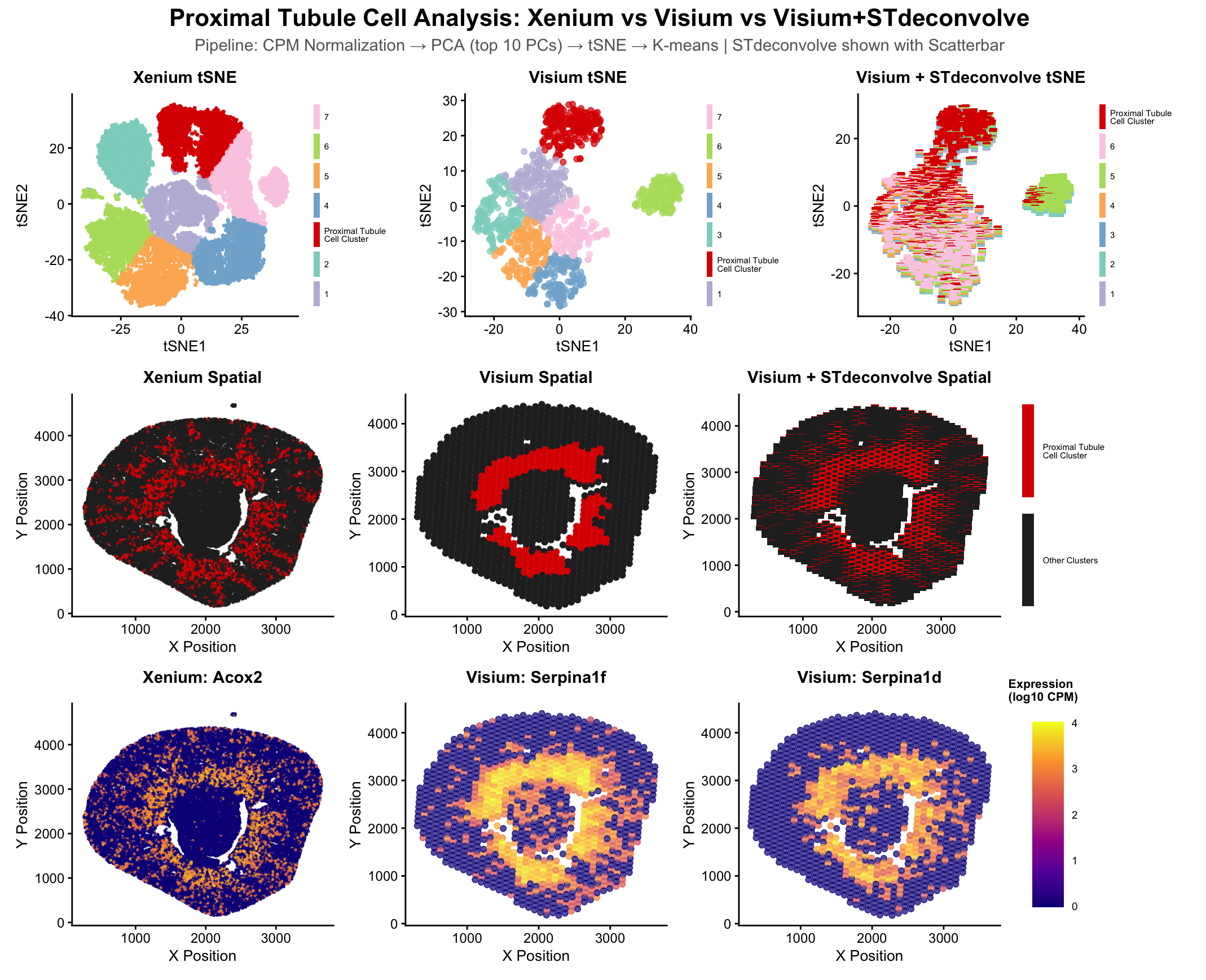
This multipanel data visualization displays the tSNE and spatial clustering of the proximal tubule cell type in serial podocyte tissue sections using gene expression data from the Xenium, Visium, and Visium-derived STDeconvolve datasets, along with the spatial expression of key differentially upregulated genes (Acox2, Serpina 1f, and Serpina 1d) in the proximal tubule cell type clusters in the Xenium and Visium datasets.

The Xenium and Visium datasets, gene expression was normalized using library size, PCA dimensionality reduction was performed, then a tSNE dimensionality reduction was performed on the top 10 PCs, then k-means clustering with k=7 was performed on the tSNE data. This process was repeated on the Visium data, except STDeconvolve was deployed to record mixed cell representation with k=7. K=7 was chosen for the visualization of all three datasets because this was the optimal k-value determined from the scree plot in homework 4, and the researcher wished to maintain a consistent k value across all visualizations to simplify comparison between them.

The first row of visualizations show the clusters for each of the three datasets in tSNE space. In each, a bright red hue is assigned to the cluster corresponding to proximal tubule cells (as determined in HW3&4), while the hues of the other clusters are assigned randomly. While the Visium tSNE plot shows well-separated clusters, the STDeconvolve data shows a little more heterogeneity in the cell types within each cell-capture spot in the Visium dataset, implying further cluster segmentation could be plausible.

The second row of visualizations isolated the proximal tubule cell cluster in the same bright red hue as in the first row (for visual continuity), while assigning all other clusters the color black in a spatial plot. These visualizations are intended to clearly show the similarity and differences between the spatial distribution of the proximal tubule cell type in the serial sections of the podocyte tissue sample. While the Visium (middle) spatial visualization displays these cells confined to a “donut-shaped” ring in the center of the cell, the STDeconvolve closely mirrors and validates the rays or streaks coming from this central ring and extending to the outward edges of the tissue section that are displayed in the cluster derived from the Xenium dataset.

The third row of visualizations shows the spatial gene expression of Acox2 (one of the top differentially expressed genes in the cluster of interest in the Xenium dataset, see HW3) in the Xenium dataset, along with the spatial gene expression of Serpina1f and Serpina1d (two of the top differentially expressed genes in the cluster of interest in the Visium dataset, see HW4). It is interesting to note that as individual gene expressions rather than greater clusters, all three genes show higher gene expressions in the “donut and outward rays” shape discussed in the paragraph before, although this pattern is shown to a greater degree in the Xenium dataset which has smaller-than-multicellular resolution. It is interesting to note however that Serpina1f and Serpina1d do display a similar pattern to a lesser degree, despite being from the Visium dataset (which is restricted to multicellular resolution).

Code

# ============================================================
# PROXIMAL TUBULE CELL ANALYSIS: XENIUM VS VISIUM VS VISIUM+STDECONVOLVE
# ============================================================
#
# PROMPTS USED TO CREATE THIS VISUALIZATION (Credit: Claude, Anthropic):
#
# 1. "Multi-panel visualization with:
#    - First row: tSNE plots for Xenium, Visium, and Visium with STdeconvolve
#    - Second row: Spatial plots showing PT cluster highlighted
#    - Third row: Spatial plot of Acox2 for Xenium, top 2 differentially
#      expressed genes for Visium (color indicates gene expression)
#    Pipeline: CPM normalization → PCA → tSNE (top 10 PCs) → K-means clustering
#    Data normalized with CPM (counts per million).
#    Proximal tubule cells identified as cluster of interest."
#
# 2. "make the central graph non translucent"
#
# 3. "make the graph color for the other category in row 2: #FFF9FB"
#
# 4. "actually this: #D3D4D9; and make sure that all the top graphs have
#    the PT cluster as red, and make sure the legend names are not cutoff
#    for the PT clusters"
#
# 5. "the clusters for proximal tubule on the top 3 graphs are not all red,
#    even though they should be"
#
# 6. "no no. the problem is that for each of the graphs on the top row,
#    i want you to find the cluster for the proximal tubule cell and
#    make sure that its color is red"
#
# 7. "make the middle row black for other clusters again"
#
# VISUALIZATION NOTES:
# - Row 1: Show ALL clusters with distinct colors (PT = RED #DC0000)
# - Row 2: PT cluster in RED, all others in BLACK (#262626)
# - Row 3: Gene expression with plasma colormap
# - STdeconvolve plots use SCATTERBAR to show cell type proportions
# - Legends use scale_fill_identity() for correct color mapping
# - PT cluster identified independently in each dataset by highest Acox2 expression
#
# ============================================================

# ============================================================
# PART 1: LOAD LIBRARIES
# ============================================================

library(ggplot2)
library(patchwork)
library(Rtsne)
library(STdeconvolve)
library(scatterbar)

# ============================================================
# PART 2: XENIUM DATA PROCESSING
# ============================================================

cat("Processing Xenium data...\n")

# Read Xenium data
xenium_data <- read.csv('/Users/henryaceves/Desktop/JHU/S2/GDV/GDV datasets/Xenium-IRI-ShamR_matrix.csv.gz')

# Build position and expression data frames
xenium_pos <- xenium_data[, c('x', 'y')]
rownames(xenium_pos) <- xenium_data[, 1]
xenium_gexp <- xenium_data[, 4:ncol(xenium_data)]
rownames(xenium_gexp) <- xenium_data[, 1]

cat(paste("Original Xenium cells:", nrow(xenium_gexp), "\n"))

# Subsample if dataset is too large (for computational efficiency)
max_cells <- 30000
if (nrow(xenium_gexp) > max_cells) {
  set.seed(123)
  sample_idx <- sample(1:nrow(xenium_gexp), size = max_cells)
  xenium_gexp <- xenium_gexp[sample_idx, ]
  xenium_pos <- xenium_pos[sample_idx, ]
  cat(paste("Subsampled to:", nrow(xenium_gexp), "cells\n"))
}

# CPM Normalization (Counts Per Million + log transformation)
xenium_totgexp <- rowSums(xenium_gexp)
xenium_mat <- log10(xenium_gexp / xenium_totgexp * 1e6 + 1)

# PCA on normalized data
cat("Running PCA on Xenium...\n")
xenium_pcs <- prcomp(xenium_mat, center = TRUE, scale = FALSE)
xenium_toppcs <- xenium_pcs$x[, 1:10]

# tSNE on top 10 PCs
cat("Running tSNE on Xenium...\n")
set.seed(123)
xenium_tsne <- Rtsne(xenium_toppcs, dims = 2, perplexity = 30, verbose = FALSE, check_duplicates = FALSE)
xenium_tsne_coords <- xenium_tsne$Y

# K-means clustering on tSNE coordinates
cat("Running k-means on Xenium...\n")
set.seed(123)
xenium_clusters <- as.character(
  kmeans(xenium_tsne_coords, centers = 7, nstart = 25, iter.max = 100, algorithm = "Lloyd")$cluster
)

# Create Xenium data frame
xenium_df <- data.frame(
  tSNE1 = xenium_tsne_coords[, 1],
  tSNE2 = xenium_tsne_coords[, 2],
  x = xenium_pos$x,
  y = xenium_pos$y,
  cluster = xenium_clusters
)
rownames(xenium_df) <- rownames(xenium_pos)

# ============================================================
# PART 3: VISIUM DATA PROCESSING
# ============================================================

cat("\nProcessing Visium data...\n")

# Read Visium data
visium_data <- read.csv('/Users/henryaceves/genomic-data-visualization-2026/data/Visium-IRI-ShamR_matrix.csv.gz')

# Build position and expression data frames
visium_pos <- visium_data[, c('x', 'y')]
rownames(visium_pos) <- visium_data[, 1]
visium_gexp <- visium_data[, 4:ncol(visium_data)]
rownames(visium_gexp) <- visium_data[, 1]

cat(paste("Visium spots:", nrow(visium_gexp), "\n"))

# CPM Normalization (Counts Per Million + log transformation)
visium_totgexp <- rowSums(visium_gexp)
visium_mat <- log10(visium_gexp / visium_totgexp * 1e6 + 1)

# PCA on normalized data
cat("Running PCA on Visium...\n")
visium_pcs <- prcomp(visium_mat, center = TRUE, scale = FALSE)
visium_toppcs <- visium_pcs$x[, 1:10]

# tSNE on top 10 PCs
cat("Running tSNE on Visium...\n")
set.seed(123)
visium_tsne <- Rtsne(visium_toppcs, dims = 2, perplexity = 30, verbose = FALSE, check_duplicates = FALSE)
visium_tsne_coords <- visium_tsne$Y

# K-means clustering on tSNE coordinates
cat("Running k-means on Visium...\n")
set.seed(123)
visium_clusters <- as.character(
  kmeans(visium_tsne_coords, centers = 7, nstart = 25, iter.max = 100, algorithm = "Lloyd")$cluster
)

# Create Visium data frame
visium_df <- data.frame(
  tSNE1 = visium_tsne_coords[, 1],
  tSNE2 = visium_tsne_coords[, 2],
  x = visium_pos$x,
  y = visium_pos$y,
  cluster = visium_clusters
)
rownames(visium_df) <- rownames(visium_pos)

# ============================================================
# PART 4: IDENTIFY PT CLUSTERS AND RUN DIFFERENTIAL EXPRESSION
# ============================================================

cat("\nIdentifying Proximal Tubule clusters...\n")

# Xenium PT cluster (highest Acox2 expression)
xenium_acox2_by_cluster <- sapply(unique(xenium_df$cluster), function(cl) {
  cells <- rownames(xenium_df)[xenium_df$cluster == cl]
  mean(xenium_mat[cells, "Acox2"])
})
names(xenium_acox2_by_cluster) <- unique(xenium_df$cluster)
xenium_pt_cluster <- names(which.max(xenium_acox2_by_cluster))
cat(paste("Xenium PT cluster:", xenium_pt_cluster, "\n"))

# Visium PT cluster (highest Acox2 expression)
visium_acox2_by_cluster <- sapply(unique(visium_df$cluster), function(cl) {
  spots <- rownames(visium_df)[visium_df$cluster == cl]
  mean(visium_mat[spots, "Acox2"])
})
names(visium_acox2_by_cluster) <- unique(visium_df$cluster)
visium_pt_cluster <- names(which.max(visium_acox2_by_cluster))
cat(paste("Visium PT cluster:", visium_pt_cluster, "\n"))

# Differential expression for Visium PT cluster
cat("Running differential expression for Visium...\n")
visium_clusterofinterest <- rownames(visium_df)[visium_df$cluster == visium_pt_cluster]
visium_othercells <- rownames(visium_df)[visium_df$cluster != visium_pt_cluster]

visium_de <- sapply(colnames(visium_mat), function(gene) {
  x1 <- visium_mat[visium_clusterofinterest, gene]
  x2 <- visium_mat[visium_othercells, gene]
  wilcox.test(x1, x2, alternative = 'greater')$p.value
})

visium_top2_genes <- names(sort(visium_de))[1:2]
cat(paste("Top 2 Visium DE genes:", paste(visium_top2_genes, collapse = ", "), "\n"))

# ============================================================
# PART 5: VISIUM WITH STDECONVOLVE
# ============================================================

cat("\nRunning STdeconvolve on Visium...\n")

# Run STdeconvolve on Visium data (using raw counts)
visium_ldas <- fitLDA(as.matrix(visium_gexp), Ks = c(7))
visium_optLDA <- optimalModel(models = visium_ldas, opt = "min")
visium_results <- getBetaTheta(visium_optLDA, perc.filt = 0.05, betaScale = 1000)

# Get deconvolution proportions (theta)
visium_decon_theta <- visium_results$theta

# Align data
common_spots <- intersect(rownames(visium_pos), rownames(visium_decon_theta))
visium_decon_pos <- visium_pos[common_spots, ]
visium_decon_theta_aligned <- visium_decon_theta[common_spots, ]
visium_decon_mat <- visium_mat[common_spots, ]

# Rename columns to Topic 1, Topic 2, etc.
colnames(visium_decon_theta_aligned) <- paste0("Topic_", 1:ncol(visium_decon_theta_aligned))

# Convert to data frame for scatterbar
visium_decon_theta_df <- as.data.frame(visium_decon_theta_aligned)

# Create position data frames for scatterbar
visium_decon_tsne_pos <- data.frame(
  x = visium_tsne_coords[match(common_spots, rownames(visium_df)), 1],
  y = visium_tsne_coords[match(common_spots, rownames(visium_df)), 2],
  row.names = common_spots
)

visium_decon_spatial_pos <- data.frame(
  x = visium_decon_pos$x,
  y = visium_decon_pos$y,
  row.names = common_spots
)

# Find PT topic in STdeconvolve (highest correlation with Acox2)
acox2_expr_decon <- visium_mat[rownames(visium_decon_theta_df), "Acox2"]
topic_acox2_cor <- sapply(colnames(visium_decon_theta_df), function(tp) {
  cor(visium_decon_theta_df[, tp], acox2_expr_decon)
})
pt_topic_name <- names(which.max(topic_acox2_cor))
cat(paste("STdeconvolve PT topic:", pt_topic_name, "\n"))

# Calculate bar sizes for scatterbar
tsne_x_range <- diff(range(visium_decon_tsne_pos$x))
tsne_y_range <- diff(range(visium_decon_tsne_pos$y))
tsne_bar_size <- min(tsne_x_range, tsne_y_range) / sqrt(nrow(visium_decon_tsne_pos)) * 1.5

spatial_x_range <- diff(range(visium_decon_spatial_pos$x))
spatial_y_range <- diff(range(visium_decon_spatial_pos$y))
spatial_bar_size <- min(spatial_x_range, spatial_y_range) / sqrt(nrow(visium_decon_spatial_pos)) * 1.2

# ============================================================
# PART 6: BUILD COLOR PALETTES
# ============================================================

cat("\nBuilding color palettes...\n")

# Base colors
pt_color <- "#DC0000"        # Proximal Tubule always RED
other_color <- "#262626"     # Black for row 2 non-PT clusters
other_colors_palette <- c("#BEBADA", "#8DD3C7", "#80B1D3", "#FDB462", "#B3DE69", "#FCCDE5")

# ----- XENIUM COLORS -----
xenium_all_clusters <- sort(as.numeric(unique(xenium_df$cluster)))
xenium_all_clusters <- as.character(xenium_all_clusters)
xenium_row1_colors <- character(length(xenium_all_clusters))
names(xenium_row1_colors) <- xenium_all_clusters

other_idx <- 1
for (i in seq_along(xenium_all_clusters)) {
  cl <- xenium_all_clusters[i]
  if (identical(cl, xenium_pt_cluster)) {
    xenium_row1_colors[i] <- pt_color
  } else {
    xenium_row1_colors[i] <- other_colors_palette[other_idx]
    other_idx <- other_idx + 1
  }
}
names(xenium_row1_colors) <- xenium_all_clusters

# ----- VISIUM COLORS -----
visium_all_clusters <- sort(as.numeric(unique(visium_df$cluster)))
visium_all_clusters <- as.character(visium_all_clusters)
visium_row1_colors <- character(length(visium_all_clusters))
names(visium_row1_colors) <- visium_all_clusters

other_idx <- 1
for (i in seq_along(visium_all_clusters)) {
  cl <- visium_all_clusters[i]
  if (identical(cl, visium_pt_cluster)) {
    visium_row1_colors[i] <- pt_color
  } else {
    visium_row1_colors[i] <- other_colors_palette[other_idx]
    other_idx <- other_idx + 1
  }
}
names(visium_row1_colors) <- visium_all_clusters

# ----- STDECONVOLVE COLORS -----
decon_all_topics <- colnames(visium_decon_theta_df)
decon_row1_colors <- character(length(decon_all_topics))
names(decon_row1_colors) <- decon_all_topics

other_idx <- 1
for (i in seq_along(decon_all_topics)) {
  tp <- decon_all_topics[i]
  if (identical(tp, pt_topic_name)) {
    decon_row1_colors[i] <- pt_color
  } else {
    decon_row1_colors[i] <- other_colors_palette[other_idx]
    other_idx <- other_idx + 1
  }
}
names(decon_row1_colors) <- decon_all_topics

# ----- ROW 2 COLORS (PT = red, others = black) -----
xenium_row2_colors <- ifelse(xenium_all_clusters == xenium_pt_cluster, pt_color, other_color)
names(xenium_row2_colors) <- xenium_all_clusters

visium_row2_colors <- ifelse(visium_all_clusters == visium_pt_cluster, pt_color, other_color)
names(visium_row2_colors) <- visium_all_clusters

decon_row2_colors <- ifelse(decon_all_topics == pt_topic_name, pt_color, other_color)
names(decon_row2_colors) <- decon_all_topics

# ============================================================
# PART 7: COMMON THEME
# ============================================================

common_theme <- theme_classic() +
  theme(
    plot.title = element_text(hjust = 0.5, face = "bold", size = 11),
    axis.text = element_text(color = "black", size = 9),
    axis.title = element_text(size = 10),
    legend.position = "none"
  )

# ============================================================
# PART 8: CREATE ROW 1 - tSNE PLOTS
# ============================================================

cat("Creating Row 1: tSNE plots...\n")

p1a <- ggplot(xenium_df, aes(x = tSNE1, y = tSNE2, col = cluster)) +
  geom_point(size = 0.5, alpha = 0.7) +
  scale_color_manual(values = xenium_row1_colors) +
  labs(title = "Xenium tSNE", x = "tSNE1", y = "tSNE2") +
  common_theme

p1b <- ggplot(visium_df, aes(x = tSNE1, y = tSNE2, col = cluster)) +
  geom_point(size = 1.5, alpha = 0.7) +
  scale_color_manual(values = visium_row1_colors) +
  labs(title = "Visium tSNE", x = "tSNE1", y = "tSNE2") +
  common_theme

p1c <- scatterbar(
  visium_decon_theta_df,
  visium_decon_tsne_pos,
  size_x = tsne_bar_size,
  size_y = tsne_bar_size
) +
  scale_fill_manual(values = decon_row1_colors) +
  labs(title = "Visium + STdeconvolve tSNE", x = "tSNE1", y = "tSNE2") +
  common_theme

# ============================================================
# PART 9: CREATE ROW 2 - SPATIAL PLOTS (PT = red, others = black)
# ============================================================

cat("Creating Row 2: Spatial plots...\n")

p2a <- ggplot(xenium_df, aes(x = x, y = y, col = cluster)) +
  geom_point(size = 0.3, alpha = 0.7) +
  scale_color_manual(values = xenium_row2_colors) +
  labs(title = "Xenium Spatial", x = "X Position", y = "Y Position") +
  common_theme

# Visium spatial - non-translucent (alpha = 1)
p2b <- ggplot(visium_df, aes(x = x, y = y, col = cluster)) +
  geom_point(size = 1.5, alpha = 1) +
  scale_color_manual(values = visium_row2_colors) +
  labs(title = "Visium Spatial", x = "X Position", y = "Y Position") +
  common_theme

p2c <- scatterbar(
  visium_decon_theta_df,
  visium_decon_spatial_pos,
  size_x = spatial_bar_size,
  size_y = spatial_bar_size
) +
  scale_fill_manual(values = decon_row2_colors) +
  labs(title = "Visium + STdeconvolve Spatial", x = "X Position", y = "Y Position") +
  common_theme

# ============================================================
# PART 10: CREATE ROW 3 - GENE EXPRESSION PLOTS
# ============================================================

cat("Creating Row 3: Gene expression plots...\n")

xenium_df$Acox2 <- xenium_mat[rownames(xenium_df), "Acox2"]

p3a <- ggplot(xenium_df, aes(x = x, y = y, col = Acox2)) +
  geom_point(size = 0.3, alpha = 0.7) +
  scale_color_viridis_c(option = "plasma") +
  labs(title = "Xenium: Acox2", x = "X Position", y = "Y Position") +
  common_theme

visium_df$gene1 <- visium_mat[rownames(visium_df), visium_top2_genes[1]]

p3b <- ggplot(visium_df, aes(x = x, y = y, col = gene1)) +
  geom_point(size = 1.5, alpha = 0.7) +
  scale_color_viridis_c(option = "plasma") +
  labs(title = paste0("Visium: ", visium_top2_genes[1]), x = "X Position", y = "Y Position") +
  common_theme

visium_df$gene2 <- visium_mat[rownames(visium_df), visium_top2_genes[2]]

p3c <- ggplot(visium_df, aes(x = x, y = y, col = gene2)) +
  geom_point(size = 1.5, alpha = 0.7) +
  scale_color_viridis_c(option = "plasma") +
  labs(title = paste0("Visium: ", visium_top2_genes[2]), x = "X Position", y = "Y Position") +
  common_theme

# ============================================================
# PART 11: CREATE LEGEND FUNCTION (FIXED WITH scale_fill_identity)
# ============================================================

create_row1_legend <- function(colors, pt_cluster_name, is_topic = FALSE) {
  cluster_names <- names(colors)
  n_clusters <- length(cluster_names)

  # Create display labels
  if (is_topic) {
    display_labels <- gsub("Topic_", "", cluster_names)
  } else {
    display_labels <- cluster_names
  }

  # Find PT cluster and replace its label
  pt_idx <- which(cluster_names == pt_cluster_name)
  if (length(pt_idx) > 0) {
    display_labels[pt_idx] <- "Proximal Tubule\nCell Cluster"
  }

  # Create data frame with colors mapped directly
  legend_df <- data.frame(
    y_pos = n_clusters:1,
    cluster_name = rev(cluster_names),
    display_label = rev(display_labels),
    color = rev(as.character(colors))
  )

  # Use scale_fill_identity() to map colors directly
  ggplot(legend_df, aes(x = 1, y = y_pos, fill = color)) +
    geom_tile(width = 0.2, height = 0.85) +
    geom_text(aes(x = 1.25, label = display_label), hjust = 0, size = 2.0, lineheight = 0.8) +
    scale_fill_identity() +
    xlim(0.8, 3.5) +
    theme_void() +
    theme(
      legend.position = "none",
      plot.margin = margin(0, 10, 0, 0)
    )
}

# ============================================================
# PART 12: CREATE LEGENDS
# ============================================================

cat("Creating legends...\n")

# Row 1 legends
p_xenium_legend <- create_row1_legend(xenium_row1_colors, xenium_pt_cluster, is_topic = FALSE)
p_visium_legend <- create_row1_legend(visium_row1_colors, visium_pt_cluster, is_topic = FALSE)
p_decon_legend <- create_row1_legend(decon_row1_colors, pt_topic_name, is_topic = TRUE)

# Row 2 legend (PT = red, Other = black)
row2_legend_df <- data.frame(
  y_pos = c(2, 1),
  label = c("Proximal Tubule\nCell Cluster", "Other Clusters"),
  color = c(pt_color, other_color)
)

p_row2_legend <- ggplot(row2_legend_df, aes(x = 1, y = y_pos, fill = color)) +
  geom_tile(width = 0.2, height = 0.85) +
  geom_text(aes(x = 1.25, label = label), hjust = 0, size = 2.0, lineheight = 0.8) +
  scale_fill_identity() +
  xlim(0.8, 3.5) +
  theme_void() +
  theme(
    legend.position = "none",
    plot.margin = margin(0, 10, 0, 0)
  )

# Expression legend (gradient bar)
p_expr_legend <- ggplot() +
  geom_tile(
    data = data.frame(y = seq(0, 4, length.out = 100), x = 1),
    aes(x = x, y = y, fill = y),
    width = 0.2, height = 0.05
  ) +
  scale_fill_viridis_c(option = "plasma", guide = "none") +
  geom_text(
    data = data.frame(y = c(0, 1, 2, 3, 4), label = c("0", "1", "2", "3", "4")),
    aes(x = 1.15, y = y, label = label),
    hjust = 0, size = 2.5
  ) +
  xlim(0.8, 1.8) +
  ylim(-0.2, 4.2) +
  labs(title = "Expression\n(log10 CPM)") +
  theme_void() +
  theme(
    plot.title = element_text(face = "bold", size = 8, hjust = 0),
    legend.position = "none"
  )

# ============================================================
# PART 13: ASSEMBLE FINAL PLOT
# ============================================================

cat("Assembling final plot...\n")

# Row 1: tSNE plots with individual legends
row1 <- (p1a | p_xenium_legend | p1b | p_visium_legend | p1c | p_decon_legend) +
  plot_layout(widths = c(3, 1.2, 3, 1.2, 3, 1.2))

# Row 2: Spatial plots with single shared legend
row2 <- (p2a | p2b | p2c | p_row2_legend) +
  plot_layout(widths = c(3, 3, 3, 2))

# Row 3: Gene expression plots with expression legend
row3 <- (p3a | p3b | p3c | p_expr_legend) +
  plot_layout(widths = c(3, 3, 3, 2))

# Combine all rows
final_plot <- (row1 / row2 / row3) +
  plot_layout(heights = c(1, 1, 1)) +
  plot_annotation(
    title = "Proximal Tubule Cell Analysis: Xenium vs Visium vs Visium+STdeconvolve",
    subtitle = "Pipeline: CPM Normalization → PCA (top 10 PCs) → tSNE → K-means | STdeconvolve shown with Scatterbar",
    theme = theme(
      plot.title = element_text(hjust = 0.5, face = "bold", size = 16),
      plot.subtitle = element_text(hjust = 0.5, size = 11, color = "gray40")
    )
  )

# Display the final plot
print(final_plot)

# ============================================================
# PART 14: SUMMARY OUTPUT
# ============================================================

cat("\n========================================\n")
cat("ANALYSIS SUMMARY\n")
cat("========================================\n")
cat("\nPIPELINE: CPM → PCA (10 PCs) → tSNE → K-means (7 clusters)\n")
cat("STdeconvolve visualized with SCATTERBAR\n")

cat("\nROW 1 (tSNE): All clusters shown with distinct colors\n")
cat("  - PT cluster is RED (#DC0000) in all three plots\n")

cat("\nROW 2 (Spatial): PT in RED (#DC0000), all others in BLACK (#262626)\n")
cat("  - Visium Spatial (center) is NON-TRANSLUCENT (alpha=1)\n")

cat("\nROW 3 (Expression): Plasma colormap showing gene expression\n")

cat("\nPROXIMAL TUBULE IDENTIFICATION (RED in all plots):\n")
cat(paste("  Xenium PT cluster:", xenium_pt_cluster, "\n"))
cat(paste("  Visium PT cluster:", visium_pt_cluster, "\n"))
cat(paste("  STdeconvolve PT topic:", pt_topic_name, "\n"))

cat("\nDATA SUMMARY:\n")
cat(paste("  Xenium cells analyzed:", nrow(xenium_df), "\n"))
cat(paste("  Xenium PT cells:", sum(xenium_df$cluster == xenium_pt_cluster), "\n"))
cat(paste("  Visium spots analyzed:", nrow(visium_df), "\n"))
cat(paste("  Visium PT spots:", sum(visium_df$cluster == visium_pt_cluster), "\n"))
cat(paste("  Visium top DE genes:", paste(visium_top2_genes, collapse = ", "), "\n"))
cat(paste("  STdeconvolve spots:", nrow(visium_decon_spatial_pos), "\n"))
cat(paste("  STdeconvolve topics:", ncol(visium_decon_theta_df), "\n"))

cat("\nCOLOR VERIFICATION:\n")
cat(paste("  Xenium cluster", xenium_pt_cluster, "color:", xenium_row1_colors[xenium_pt_cluster], "\n"))
cat(paste("  Visium cluster", visium_pt_cluster, "color:", visium_row1_colors[visium_pt_cluster], "\n"))
cat(paste("  STdeconvolve", pt_topic_name, "color:", decon_row1_colors[pt_topic_name], "\n"))
cat("========================================\n")

01 Mar 2026

HW EC2

« EC1-How Normalization and Log Transformation Reshape PCA Geometry in Gene Expression Data Using animation to visualize the importance of data normalization and log-transformation for quality control »