Deconvolution and Multi-Modal Comparison of the Renal S3 Segment
Note, the png is named “EC2_ooni5.png”, as a desired name was not specified in the HW powerpoint.
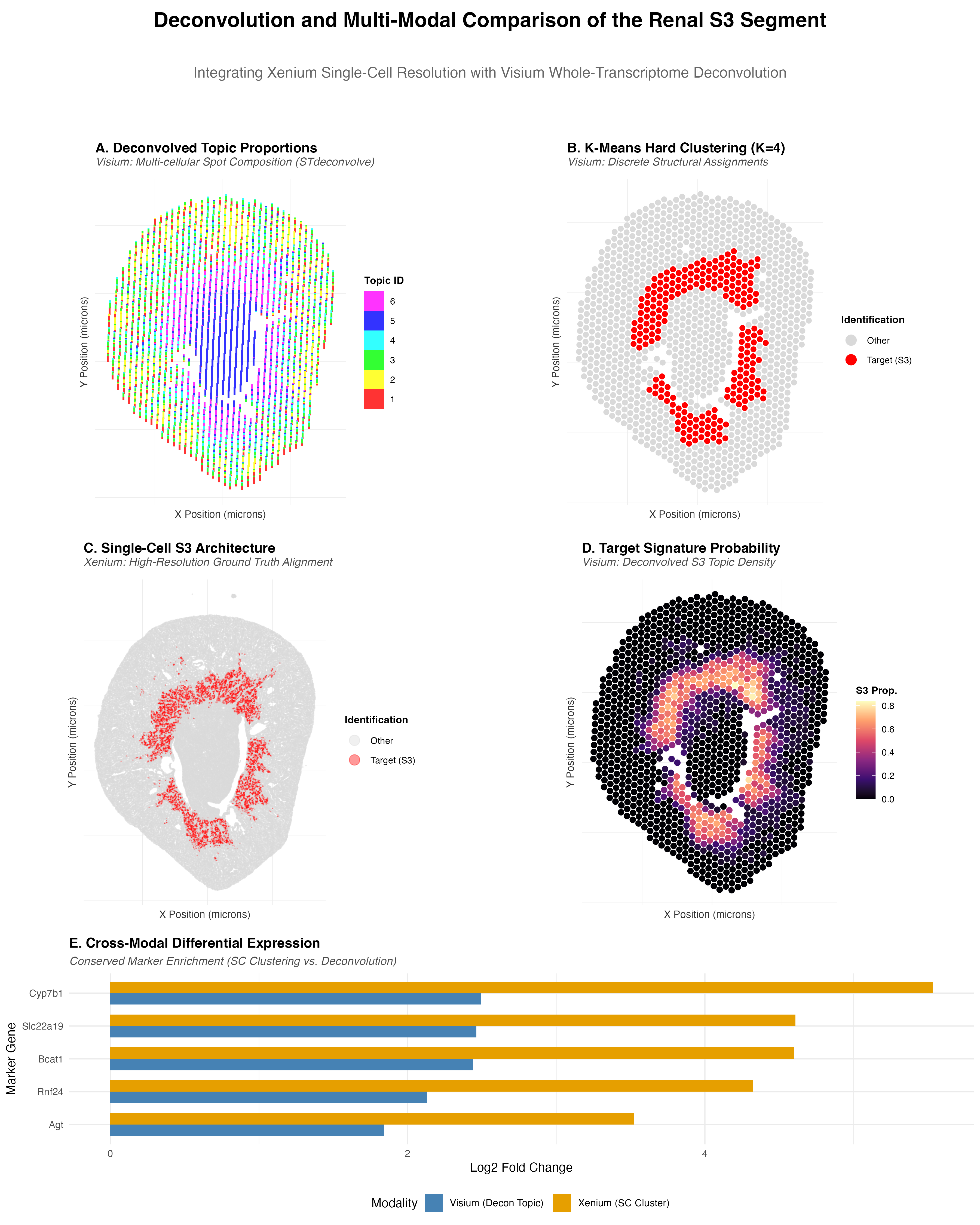
Figure Description
- Panel A (STdeconvolve): Visualizes the proportions of deconvolved cell-type signatures within each Visium spot using a scatterbar plot. This reveals the transcriptomic heterogeneity hidden within the 55µm multi-cellular spots, and the tracked S3 structure can be identified.
- Panel B (K-means): Displays discrete cluster assignments (K=4) for the Visium tissue, replicating the hard-boundary mapping performed in HW4.
- Panels C & D (Cross-Modality Spatial Map): Provide a side-by-side comparison of the S3 segment. Panel C shows the single-cell ground truth from Xenium clustering (HW3), while Panel D shows the continuous probability gradient of the deconvolved S3 topic in Visium. The S3 segment in both modalities was identified by isolating the cluster (Xenium) and deconvolved topic (Visium) exhibiting the highest average expression of the marker gene Cyp7b1 (oxysterol 7-alpha-hydroxylase).
- Panel E (Differential Expression): A comparative bar chart demonstrating the conserved upregulation of key marker genes (e.g., Cyp7b1, Slc22a19) across both technologies, validating the deconvolution results. The high Log2 Fold Change of Cyp7b1 and Slc22a19 in both modalities demonstrates that the transcriptomic signature of the proximal tubule S3 segment is conserved across platforms, providing cross-modal validation of the deconvolution results.
Comparison of Results
The current deconvolution analysis provides an improvement over the previous clustering-only approaches. In HW4 (Visium K-means), the S3 segment was represented by a discrete, “blocky” cluster. While this correctly identified the general anatomical location (cortex-medulla boundary), it failed to account for spots containing mixtures of cell types. The STdeconvolve results (Panel A and D), however, resolve this “blurriness.” The proportional signatures allow us to see how the S3 segment actually tapers off and mixes with adjacent tissues, providing a much closer approximation to the high-resolution single-cell data from HW3 (Xenium). While Xenium provides absolute spatial precision, the deconvolution of whole-transcriptome Visium data allows us to discover these same boundaries and conserved marker sets (Panel E) in an unbiased manner.
5. Code (paste your code in between the ``` symbols)
.
  library(Seurat)
  library(data.table)
  library(dplyr)
  library(ggplot2)
  library(patchwork)
  library(STdeconvolve)
  library(scatterpie)
  library(cowplot)
  library(viridis)
})

set.seed(42)

# =============================================================================
# PART 1: VISIUM ANALYSIS (HW 4 Logic)
# =============================================================================

#From HW 4:
# -----------------------------------------------------------------------------
# User-facing analysis settings
# -----------------------------------------------------------------------------
#Prompt to set pcs at 10 and 4 based on elbow graph data. Remaining analysis carried out similar to with Xenium data.
data_path_vis <- "Visium-IRI-ShamR_matrix.csv"
my_gene <- "Cyp7b1"
n_pcs_vis <- 10           # Optimized for Visium
k_vis <- 4                # Optimized for Visium

# -----------------------------------------------------------------------------
# Section 1 & 2: Data Loading and Seurat Object Creation
# -----------------------------------------------------------------------------
data_raw_vis <- fread(data_path_vis)
counts_vis <- t(as.matrix(data_raw_vis[, -(1:3)]))
colnames(counts_vis) <- data_raw_vis[[1]]
sham_vis <- CreateSeuratObject(counts = counts_vis, project = "ShamR_Visium")

# Map coordinates directly from the Visium matrix
sham_vis$x <- data_raw_vis$x
sham_vis$y <- data_raw_vis$y

# -----------------------------------------------------------------------------
# Section 3: Normalization, Scaling, and Dimensionality Reduction
# -----------------------------------------------------------------------------
sham_vis <- NormalizeData(sham_vis)
sham_vis <- FindVariableFeatures(sham_vis)
sham_vis <- ScaleData(sham_vis, features = VariableFeatures(sham_vis))
sham_vis <- RunPCA(sham_vis, features = VariableFeatures(sham_vis), npcs = 30)

# -----------------------------------------------------------------------------
# Section 4 & 5: Clustering, t-SNE, and Marker Discovery
# -----------------------------------------------------------------------------
pca_embeddings_vis <- Embeddings(sham_vis, reduction = "pca")[, 1:n_pcs_vis]
final_kmeans_vis <- kmeans(pca_embeddings_vis, centers = k_vis, nstart = 25)
sham_vis$kmeans_clusters <- factor(final_kmeans_vis$cluster)
Idents(sham_vis) <- "kmeans_clusters"

# Identify the target cluster for the S3 segment
target_cluster_vis <- names(which.max(tapply(FetchData(sham_vis, vars = my_gene)[[1]], Idents(sham_vis), mean)))

sham_vis <- RunTSNE(sham_vis, dims = 1:n_pcs_vis)
markers_vis <- FindAllMarkers(sham_vis, only.pos = TRUE, test.use = "wilcox")

#prompt defined desired gene, search which cluster it belongs to.
target_cluster_vis <- names(which.max(tapply(FetchData(sham_vis, vars = my_gene)[[1]], Idents(sham_vis), mean)))
print(target_cluster_vis)


# =============================================================================
# PART 2: XENIUM ANALYSIS (HW 3 Logic)
# =============================================================================

#From HW 3:
# -----------------------------------------------------------------------------
# User-facing analysis settings
# -----------------------------------------------------------------------------
data_path_xen <- "Xenium-IRI-ShamR_matrix.csv"
# my_cluster <- "2"    <-- Commented out: we will calculate this dynamically below to match Visium logic
my_gene <- "Cyp7b1"    # Swapped to the new #1 marker for Cluster 2
n_pcs_xen <- 17        # Determined from PCA elbow plot
k_xen <- 8             # Determined from K-means WSS elbow plot

# -----------------------------------------------------------------------------
# Section 1 & 2: Data Loading and Seurat Object Creation
# -----------------------------------------------------------------------------
data_raw_xen <- fread(data_path_xen)
counts_xen <- t(as.matrix(data_raw_xen[, -(1:3)]))
colnames(counts_xen) <- data_raw_xen$V1
sham_xen <- CreateSeuratObject(counts = counts_xen, project = "ShamR")

# -- Strict Coordinate Matching
current_cells <- Cells(sham_xen)
match_indices <- match(current_cells, data_raw_xen$V1)
sham_xen$x <- data_raw_xen$x[match_indices]
sham_xen$y <- data_raw_xen$y[match_indices]
sham_xen <- subset(sham_xen, cells = Cells(sham_xen)[!is.na(sham_xen$x)])

# -----------------------------------------------------------------------------
# Section 3: Normalization, Scaling, and Dimensionality Reduction
# -----------------------------------------------------------------------------
sham_xen <- NormalizeData(sham_xen)
sham_xen <- FindVariableFeatures(sham_xen)
sham_xen <- ScaleData(sham_xen, features = VariableFeatures(sham_xen))
sham_xen <- RunPCA(sham_xen, features = VariableFeatures(sham_xen), npcs = 50)

# -----------------------------------------------------------------------------
# Tuning Plots (Commented Out)
# This block was used to determine the optimal `n_pcs` and `k_clusters` values.
# It is commented out because these are intermediate steps, not part of the
# final reported figure. We keep the code here to document our process.
# -----------------------------------------------------------------------------
if (FALSE) {
  # PCA elbow plot
  print(ElbowPlot(sham_xen, ndims = 50))

  # K-means WSS elbow plot
  pca_embeddings_test <- Embeddings(sham_xen, reduction = "pca")[, 1:n_pcs_xen]
  wss <- sapply(1:20, function(k){
    kmeans(pca_embeddings_test, centers = k, nstart = 10)$tot.withinss
  })
  elbow_df <- data.frame(k = 1:20, wss = wss)
  print(ggplot(elbow_df, aes(x = k, y = wss)) + geom_line() + geom_point())
}

# -----------------------------------------------------------------------------
# Section 4 & 5: Clustering, t-SNE, and Marker Discovery
# -----------------------------------------------------------------------------
#Looks like we start to get diminishing returns around PC17, so I want you to stop it there and create the PC17 plot. Then we're going to do k-means on the PCA. Again, I want you to put a graph of the various k so I can find the elbow, and then we'll choose from there and we'll move on from there, but just do this.
#It looks as though we are getting an appropriate k around 7 or 8, it seems. Now, from there, we're going to apply t-SNE in order to visualize our data properly. Then we'll do one versus the rest Wilcoxon in order to find the differentially expressed genes. So do that first, or like, just do this section now.

pca_embeddings_xen <- Embeddings(sham_xen, reduction = "pca")[, 1:n_pcs_xen]
final_kmeans_xen <- kmeans(pca_embeddings_xen, centers = k_xen, nstart = 25)
sham_xen$kmeans_clusters <- factor(final_kmeans_xen$cluster)
Idents(sham_xen) <- "kmeans_clusters"
sham_xen <- RunTSNE(sham_xen, dims = 1:n_pcs_xen)

markers_xen <- FindAllMarkers(sham_xen, only.pos = TRUE, test.use = "wilcox")

# Dynamically identify the target cluster in Xenium (matching Visium logic)
target_cluster_xen <- names(which.max(tapply(FetchData(sham_xen, vars = my_gene)[[1]], Idents(sham_xen), mean)))


if (!requireNamespace("remotes", quietly = TRUE)) install.packages("remotes")
remotes::install_github("JEFworks-Lab/scatterbar")
library(scatterbar)


# =============================================================================
# Multi-Modal Deconvolution & Comparison
# =============================================================================

#Prompt: assistance with deconvolution math required for STdeconvolve.
# 1. RUN THE DECONVOLUTION MATH
# -----------------------------------------------------------------------------
# Extract raw counts and filter
counts_vis_decon <- LayerData(sham_vis, layer = "counts")
cleaned_vis <- cleanCounts(counts_vis_decon, min.lib.size = 100, min.reads = 1)
corpus_vis <- restrictCorpus(cleaned_vis, removeAbove = 1.0, removeBelow = 0.05)

# Fit LDA and get results
ldas_vis <- fitLDA(t(as.matrix(corpus_vis)), Ks = seq(2, 6, by = 1))
opt_vis <- optimalModel(models = ldas_vis, opt = "min")
results_vis <- getBetaTheta(opt_vis)

# Extract Proportions (Theta) and Coordinates
decon_proportions <- as.data.frame(results_vis$theta)
decon_proportions$x <- sham_vis$x
decon_proportions$y <- sham_vis$y

# Identify Topic for S3 Segment (Cyp7b1)
beta_vis <- as.data.frame(results_vis$beta)
target_topic_vis <- rownames(beta_vis)[which.max(beta_vis[, my_gene])]


#Was rewritten due to troubleshooting plotting errors.


#Prompt: utilize same formatting style present in my HW 5.
# =============================================================================
# SECTION: FINAL MASTER VISUALIZATION (HW 5 GRID & LABELING STYLE)
# =============================================================================
library(cowplot)
library(viridis)
library(scatterbar)

# 1. THE "MASTER GRID" THEME
# -----------------------------------------------------------------------------
# Replicates the HW 5 technical look: Bold titles, light grids, axis buffers.
master_grid_theme <- theme_minimal() +
  theme(
    plot.title = element_text(face = "bold", size = 12, margin = margin(b = 2)),
    plot.subtitle = element_text(size = 10, face = "italic", color = "grey30", margin = margin(b = 10)),
    axis.title = element_text(size = 9, color = "grey20"),
    axis.title.x = element_text(margin = margin(t = 5)),
    axis.title.y = element_text(margin = margin(r = 5)),
    axis.text = element_blank(),
    axis.ticks = element_blank(),
    # Restoring the HW 5 technical grids
    panel.grid.major = element_line(color = "grey92", linewidth = 0.2),
    panel.grid.minor = element_blank(),
    legend.title = element_text(size = 9, face = "bold"),
    legend.text = element_text(size = 8),
    legend.position = "right",
    plot.margin = margin(10, 10, 10, 10)
  )

# 2. GENERATE INDIVIDUAL PANELS
# -----------------------------------------------------------------------------

#Prompt: Reuse panels from HW 3 and 4, create scatterbar and comparison plot—iterated many times in order to get formatting and labels correct
# --- PANEL A: Deconvolved Topic Proportions (SCATTERBAR) ---
theta_mtx <- as.matrix(decon_proportions[, !colnames(decon_proportions) %in% c("x", "y")])
pos_df <- as.data.frame(decon_proportions[, c("x", "y")])
rownames(theta_mtx) <- rownames(pos_df) <- rownames(decon_proportions)

p_a <- scatterbar::scatterbar(theta_mtx, pos_df, 28) +
  labs(title = "A. Deconvolved Topic Proportions",
       subtitle = "Visium: Multi-cellular Spot Composition (STdeconvolve)",
       x = "X Position (microns)", y = "Y Position (microns)", # Fixed axis labels
       fill = "Topic ID") +
  master_grid_theme + coord_fixed()

# --- PANEL B: Visium K-Means (Hard Clustering) ---
vis_km_df <- data.frame(x = sham_vis$x, y = sham_vis$y, Cluster = Idents(sham_vis))
p_b <- ggplot(vis_km_df, aes(x = x, y = y, color = (Cluster == target_cluster_vis))) +
  geom_point(size = 1.8) +
  scale_color_manual(values = c("TRUE" = "red", "FALSE" = "grey85"),
                     labels = c("TRUE" = "Target (S3)", "FALSE" = "Other"), name = "Identification") +
  labs(title = "B. K-Means Hard Clustering (K=4)",
       subtitle = "Visium: Discrete Structural Assignments",
       x = "X Position (microns)", y = "Y Position (microns)") +
  master_grid_theme + coord_fixed() +
  guides(color = guide_legend(override.aes = list(size = 4)))

# --- PANEL C: Xenium Target Mapping (Labled Legend added) ---
xen_sp_df <- data.frame(x = sham_xen$x, y = sham_xen$y, Cluster = Idents(sham_xen))
p_c <- ggplot(xen_sp_df, aes(x = x, y = y, color = (Cluster == target_cluster_xen))) +
  geom_point(size = 0.05, alpha = 0.4) +
  scale_color_manual(values = c("TRUE" = "red", "FALSE" = "grey85"),
                     labels = c("TRUE" = "Target (S3)", "FALSE" = "Other"), name = "Identification") +
  labs(title = "C. Single-Cell S3 Architecture",
       subtitle = "Xenium: High-Resolution Ground Truth Alignment",
       x = "X Position (microns)", y = "Y Position (microns)") +
  master_grid_theme + coord_fixed() +
  guides(color = guide_legend(override.aes = list(size = 4))) # Legend restored

# --- PANEL D: Visium Deconvolved Target Map ---
p_d <- ggplot(decon_proportions, aes(x = x, y = y, color = .data[[target_topic_vis]])) +
  geom_point(size = 2.0) +
  scale_color_viridis_c(option = "magma", name = "S3 Prop.") +
  labs(title = "D. Target Signature Probability",
       subtitle = "Visium: Deconvolved S3 Topic Density",
       x = "X Position (microns)", y = "Y Position (microns)") +
  master_grid_theme + coord_fixed()

# --- PANEL E: Cross-Modality DE Comparison ---
pot_markers <- markers_xen %>% filter(cluster == target_cluster_xen) %>% slice_max(avg_log2FC, n = 10) %>% pull(gene)
valid_markers <- intersect(pot_markers, colnames(beta_vis))
plot_markers <- head(valid_markers, 5)
vis_fc <- log2(as.numeric(beta_vis[target_topic_vis, plot_markers]) / colMeans(beta_vis[, plot_markers]))
xen_fc <- markers_xen %>% filter(cluster == target_cluster_xen, gene %in% plot_markers) %>%
  arrange(match(gene, plot_markers)) %>% pull(avg_log2FC)
comp_df <- data.frame(Gene = rep(plot_markers, 2), Log2FC = c(xen_fc, vis_fc),
                      Modality = rep(c("Xenium (SC Cluster)", "Visium (Decon Topic)"), each = length(plot_markers)))

p_e <- ggplot(comp_df, aes(x = reorder(Gene, Log2FC), y = Log2FC, fill = Modality)) +
  geom_bar(stat = "identity", position = "dodge", width = 0.7) +
  scale_fill_manual(values = c("steelblue", "#E69F00")) +
  coord_flip() + theme_minimal() +
  labs(title = "E. Cross-Modal Differential Expression",
       subtitle = "Conserved Marker Enrichment (SC Clustering vs. Deconvolution)",
       x = "Marker Gene", y = "Log2 Fold Change") +
  theme(plot.title = element_text(face = "bold", size = 12),
        plot.subtitle = element_text(size = 10, face = "italic", color = "grey30"),
        legend.position = "bottom")

# 3. ASSEMBLE GRID (ROW-BY-ROW)
# -----------------------------------------------------------------------------
row1 <- plot_grid(p_a, p_b, nrow = 1, rel_widths = c(1, 1), align = 'h', axis = 'bt')
row2 <- plot_grid(p_c, p_d, nrow = 1, rel_widths = c(1, 1), align = 'h', axis = 'bt')

main_grid <- plot_grid(row1, row2, p_e, ncol = 1, rel_heights = c(1.5, 1.5, 1.1))

# 4. HEADER CANVAS
# -----------------------------------------------------------------------------
title_canvas <- ggdraw() +
  draw_label("Deconvolution and Multi-Modal Comparison of the Renal S3 Segment",
             fontface = 'bold', size = 18, y = 0.85) +
  draw_label("Integrating Xenium Single-Cell Resolution with Visium Whole-Transcriptome Deconvolution",
             color = "grey40", size = 13, y = 0.45)

# 5. FINAL ASSEMBLY
# -----------------------------------------------------------------------------
final_panel <- plot_grid(title_canvas, main_grid, ncol = 1, rel_heights = c(0.12, 1))

print(final_panel)

# Export at high-res
ggsave("Kidney_S3_Final_Master_Panel.png",
       plot = final_panel, width = 12, height = 15, dpi = 300, bg = "white")