Deconvolution on Visium Dataset

Hi! I am Saadia Jameel, a first year BME Ph.D. student

Description

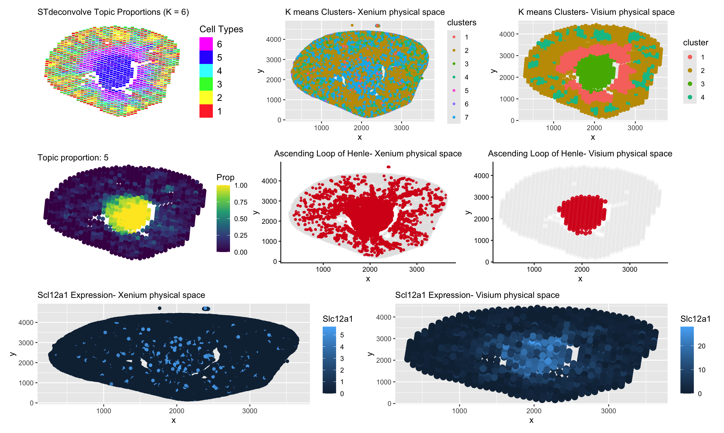
In the deconvolution analysis (Visium), the topic of interest looks very tightly concentrated in the center. Each Visium spot contains multiple cells. STdeconvolve models mixtures of transcriptional programs within each spot, so a topic only shows strong enrichment where that cell type makes up a large proportion of the spot. In the kidney, the Ascending Loop of Henle is organized in a fairly compact central region, so the deconvolved topic lights up clearly there. Outside that region, even if a few relevant cells are present, their signal gets diluted by other cell types within the same spot. As a result, the estimated proportion stays low and the enrichment looks very clean and centered.

In contrast, Xenium works at single-cell resolution. Each point is an individual cell, not a mixture. Cells from the Ascending Loop are arranged along tubular structures and can extend beyond one tightly packed area. Because clustering assigns each cell to a group independently, the cluster of interest looks more scattered and less strictly confined. What we see there is the true spatial spread of individual cells rather than an averaged signal across spots.

The same idea applies to the marker gene, Slc12a1. In Xenium, expression looks more distributed because you can detect every expressing cell wherever it sits. In Visium, expression is averaged across all cells in a spot, so strong signal only appears where many Slc12a1 positive cells are concentrated together. That makes the Visium signal look smoother and more centralized. Overall, the difference comes down to resolution, deconvolution and Visium gene expression reflect spot-level mixtures, while Xenium captures the spatial distribution of individual cells.

5. Code (paste your code in between the ``` symbols)

library(ggplot2)
library(patchwork)

require(remotes) 
remotes::install_github('JEFworks-Lab/STdeconvolve')
library(STdeconvolve)

remotes::install_github('JEFworks-Lab/scatterbar')
library(scatterbar)

# # PLAN
# 1. Load xenium and perform clustering and diff expression analysis 
# 2. Load visum and perform deconvolution and diff expression analysis
# 3. Get the interested cell type proportion of the two

# load Xenium data
data <- read.csv("~/Documents/genomic-data-visualization-2026/data/Xenium-IRI-ShamR_matrix.csv.gz")

# get the spatial positions
pos <- data[,c('x', 'y')]
rownames(pos) <- data[,1]

# get gene expression values
gexp <- data[, 4:ncol(data)]
rownames(gexp) <- data[,1]

# normalize
totgexp= rowSums(gexp)
mat <- log10(gexp/totgexp *1e6 +1)

# 2. linear dimensionality reduction
pcs <- prcomp(mat)
# visualize PC
df <- data.frame(
  pos,
  pcs$x
)

# # 3. tSNE
# ts <- Rtsne::Rtsne(pcs$x[,1:10], dim=2)
# names(ts)
# emb <- ts$Y
# df <- data.frame(
#   emb,
#   totgexp= totgexp
# )

# 4. clustering
set.seed(10) # for luster labels to remain the same throughout runs
clusters <- as.factor(kmeans(pcs$x[,1:5], centers= 7)$cluster)

# see how many cells are in each cluster
table(clusters)

df <- data.frame(
  # emb,
  pos, 
  clusters, 
  totgexp= totgexp,
  # gene=mat[,'Slc34a1'],
  pcs$x
)


# highlight cluster of interest in a different colour
# cluster_color_interest <- c(
#   "1" = "#D7191C",  # red (interest)
#   "2" = "#EEEEEE",  # light grey
#   "3" = "#EEEEEE",  # light grey
#   "4" = "#EEEEEE",  # light grey (is everywhere)
#   "5" = "#EEEEEE",  # light grey
#   "6" = "#EEEEEE",  # light grey
#   "7" = "#EEEEEE"  # light grey (everywhere)
# )

# cluster_colors <- c(
#   "1" = "#D6EAF8",  # very light blue
#   "2" = "#AED6F1",
#   "3" = "#5DADE2",
#   "4" = "#3498DB",
#   "5" = "#2E86C1",
#   "6" = "#1B4F72",
#   "7" = "#0B3C5D"   # deep navy
# )
cluster_colors <- c(
  "1" = "#F8766D",  # coral
  "2" = "#C49A00",  # mustard
  "3" = "#53B400",  # green
  "4" = "#00C094",  # teal
  "5" = "#FB61D7",  # sky blue
  "6" = "#A58AFF",  # lavender
  "7" = "#00B6EB"   # pink
)

# view clusters
clusters_xenium <- ggplot(df, aes(x=x, y=y, col=clusters))+
  geom_point(size=1)+
  scale_colour_manual(values = cluster_colors)+
  labs(
    title= "K means Clusters- Xenium physical space"
  )+
  theme(plot.title = element_text(size = 11))

clusters_xenium
# view cluster of interest
p_spatial_xenium <- ggplot() +
  geom_point(
    data = subset(df, clusters != "1"),
    aes(x = x, y = y),
    color = "#D9D9D9",
    alpha = 0.05,
    size  = 0.6
  ) +
  geom_point(
    data = subset(df, clusters == "1"),
    aes(x = x, y = y),
    color = "#D7191C",
    alpha = 0.8,
    size  = 0.9
  ) +
  labs(
    title= "Ascending Loop of Henle- Xenium physical space"
  )+
  theme_classic() +
  theme(
    plot.title = element_text(hjust = 0.5, size=11)
  )

p_spatial_xenium

# differentially expressed genes in cluster 1
# identify cluster of interest as 1
clusterofinterest_a <- names(clusters)[clusters == 1]
clusterofinterest_b <- names(clusters)[clusters != 1]

# identify differentially expressed genes
out <- sapply(colnames(mat), function(gene){
  x1 <- mat[clusterofinterest_a,gene]
  x2 <- mat[clusterofinterest_b,gene]
  wilcox.test(x1, x2, alternative = "greater")$p.value
})

# the lower the P value, the greater the relative upregulation in x1 compared to x2
sort(out, decreasing = FALSE)[1:30]

# view differentially expressed genes
df <- data.frame(
  # emb,
  pos, 
  clusters, 
  totgexp= totgexp,
  mat,
  pcs$x
)

plot_slc12a1_xenium <- ggplot(df, aes(x=x, y=y, col=Slc12a1))+geom_point()+
  labs(
    title= "Scl12a1 Expression- Xenium physical space"
  )+
  theme(plot.title = element_text(size = 11))

plot_slc12a1_xenium

plot_umod_xenium <- ggplot(df, aes(x=x, y=y, col=Umod))+geom_point()
plot_umod_xenium

# DECONVOLUTION - VISIUM (fixed)

library(STdeconvolve)

# -------------------------
# Load data
# -------------------------
data <- read.csv("~/Documents/genomic-data-visualization-2026/data/Visium-IRI-ShamR_matrix.csv.gz",
                 stringsAsFactors = FALSE)

pos <- data[,2:3]
colnames(pos) <- c('x', 'y')
cd <- data[, 4:ncol(data)]
rownames(pos) <- rownames(cd) <- data[,1]

## remove pixels with too few genes
counts <- cleanCounts(t(cd), min.lib.size = 100)

## feature select for genes
corpus <- restrictCorpus(counts, removeAbove=1.0, removeBelow = 0.05)

## choose optimal number of cell-types
ldas <- fitLDA(
  t(as.matrix(corpus)),   # input must be spots x genes
  Ks  = seq(2, 9, by = 1),
  perc.rare.thres = 0.05,
  ncores  = 8,            # adjust to your cluster
  verbose = TRUE,
  plot = TRUE
)
# ldas <- fitLDA(t(as.matrix(corpus)), Ks = c(5))

## get best model results
# optLDA <- optimalModel(models = ldas, opt = "min")
optLDA <- ldas$models[["6"]]

## extract deconvolved cell-type proportions (theta) and transcriptional profiles (beta)
results <- getBetaTheta(optLDA, perc.filt = 0.05, betaScale = 1000)
deconProp <- results$theta
deconGexp <- results$beta
# # scatterpie
# vizAllTopics(deconProp, pos,
#              r=45, lwd=0)	 


# -------------------------
# scatterbar
# -------------------------
# FIX: align pos to deconProp (cleanCounts removes some spots) + make x/y numeric
pos <- as.data.frame(pos)
pos$x <- as.numeric(pos$x)
pos$y <- as.numeric(pos$y)
pos <- pos[rownames(deconProp), , drop = FALSE]

plot_celltype_proportions <- scatterbar(
  deconProp,
  pos,
  size_x = 80,
  size_y = 80,
  legend_title = "Cell Types"
  )+
  labs(title = "STdeconvolve Topic Proportions (K = 6)")+
  theme(plot.title = element_text(size = 11))

plot_celltype_proportions
# -------------------------
# k-means on cell-type proportions
# -------------------------
set.seed(10)
theta_mat <- as.matrix(deconProp)

wss <- sapply(2:30, function(k) {
  kmeans(theta_mat, centers = k, nstart = 20)$tot.withinss
})

plot(2:30, wss, type = "b",
     xlab = "Number of clusters (k)",
     ylab = "Total within-cluster sum of squares")

set.seed(10)
k <- 4
kmeans_res <- kmeans(theta_mat, centers = k, nstart = 20)
clusters <- as.factor(kmeans_res$cluster)
names(clusters) <- rownames(theta_mat)   # add barcode names (CRUCIAL)

df_cluster <- data.frame(
  x = pos$x,
  y = pos$y,
  cluster = clusters
)

clusters_visium <- ggplot(df_cluster, aes(x = x, y = y, color = cluster)) +
  geom_point(size = 2) +
  scale_colour_manual(values = cluster_colors)+
  labs(
    title= "K means Clusters- Visium physical space"
  )+
  theme(plot.title = element_text(size = 11))

clusters_visium
# -------------------------
# visualize cluster of interest (cluster 3)
# -------------------------
cluster_id <- "3"

p_spatial_visium <- ggplot(df_cluster) +
  geom_point(
    data = subset(df_cluster, cluster != cluster_id),
    aes(x = x, y = y),
    color = "#D9D9D9",
    alpha = 0.25,
    size  = 2
  ) +
  geom_point(
    data = subset(df_cluster, cluster == cluster_id),
    aes(x = x, y = y),
    color = "#D7191C",
    alpha = 0.9,
    size  = 2
  ) +
  labs(title = paste0("Ascending Loop of Henle- Visium physical space")) +
  theme_classic() +
  theme(plot.title = element_text(hjust = 0.5, size=11))

p_spatial_visium

# -------------------------
# differential gene expression: cluster 2 vs all others
# -------------------------
clusterofinterest_a <- names(clusters)[clusters == cluster_id]
clusterofinterest_b <- names(clusters)[clusters != cluster_id]

# clusterofinterest_a <- rownames(deconProp)[5]
# clusterofinterest_b <- rownames(deconProp)[!5]

out <- sapply(colnames(cd), function(gene) {
  x1 <- cd[clusterofinterest_a, gene]
  x2 <- cd[clusterofinterest_b, gene]
  wilcox.test(x1, x2, alternative = "greater")$p.value
})

sort(out, decreasing = FALSE)[1:30]

# view differentially expressed genes
df <- data.frame(
  pos, 
  cd,
  clusters
)

plot_slc12a1_visium <- ggplot(df, aes(x=x, y=y, col=Slc12a1))+geom_point(size=3.5)+
  labs(
    title= "Scl12a1 Expression- Visium physical space"
  )+
  theme(plot.title = element_text(size = 11))

plot_slc12a1_visium

plot_umod_visium <- ggplot(df, aes(x=x, y=y, col=Umod))+geom_point()
plot_umod_visium

# (plot_celltype_proportions + clusters_xenium + clusters_visum) / (p_spatial_xenium + p_spatial_visium) / (plot_slc12a1_xenium + plot_slc12a1_visium)

# Topic 5 proportion map (aligned to deconProp like scatterbar)
df_t <- data.frame(
  pos[rownames(deconProp), , drop = FALSE],
  prop = deconProp[, 5]
)

plot_topic_5 <- ggplot(df_t, aes(x = x, y = y, color = prop)) +
  geom_point(size = 2) +
  theme_void() +
  scale_color_viridis_c() +
  labs(title = "Topic proportion: 5", color = "Prop")+
  theme(plot.title = element_text(size = 11))

plot_topic_5

final_plot <- (plot_celltype_proportions + clusters_xenium + clusters_visium) / (plot_topic_5 + p_spatial_xenium + p_spatial_visium) / (plot_slc12a1_xenium + plot_slc12a1_visium)

final_plot + plot_layout(widths = c(1,1,1))

# save.image("hwEC2.RData")

6. Resources

I used R documentation and the ? help function on R itself to understand functions.

I used AI to help organize plots better

01 Mar 2026

HW EC2

« HW EC1 Animation of Non-Linear Dimensionality Reduction (tSNE) on Varied number of PCs »