Identifying Red and White Pulp in Spleen Data

Your description should reference papers and content that allowed you to interpret your cell clusters as a particular cell-types.
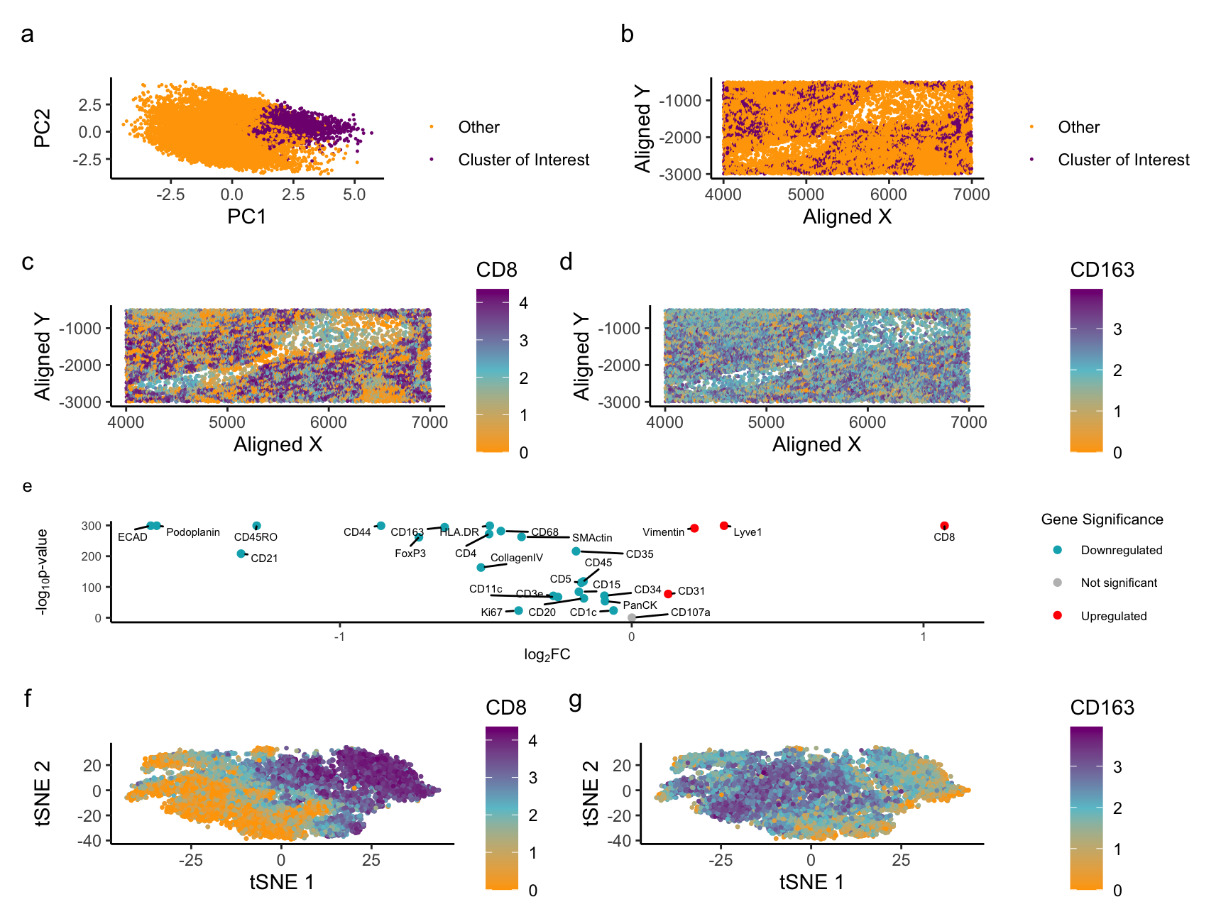
My figure visualizes the white and red pulp of the spleen. The visualization identifies two known proteins expressed in t-cells and platelet/epithelial cells. I found that white pulp mainly contains T-cells and cells related to the immune system, and red pulp mainly contains red blood cells and platelet cells.
I identified the white pulp by first normalizing my data based on protein expression in the cells. Then, I clustered the normalized protein expression in 5 clusters based on total withness. Next, I selected a known protein in T-cells/immune cells: CD8. I found which cluster CD8 was expressed the most in, and it was in clusters 4 and 1. I did the same step for the red pulp but with protein CD163, which is a known “transmembrane receptor for the hemoglobin–haptoglobin (Hb:Hp) complexes” [4]. Hemoglobin is found in red blood cells. Then, I found CD163 was expressed the most in cluster 4. I chose cluster 4 to focus on because it was the common cluster between the two proteins. Upon comparing the spatial data of both proteins being expressed against the spatial data of cluster 4, both proteins show increased expression. The t-SNE plot of CD8 also backs this up; however, it’s harder to tell in the CD163 t-SNE plot. I have identified white and red pulp tissues by linking two known proteins, each highly expressed in either immune cells or red blood cells, to the same cluster and confirming with literature that these proteins are expressed in white and red pulp tissues.
Sources:
- https://www.biostat.jhsph.edu/~kkammers/software/CVproteomics/R_guide.html
- https://zoomify.luc.edu/lymphoid/dms122/popup.html # mentions white is t-cells- macrophages
- https://www.sigmaaldrich.com/US/en/product/sigma/c2562 # epitheial cells
- https://www.sciencedirect.com/topics/biochemistry-genetics-and-molecular-biology/cd163#:~:text=CD163%20is%20an%20acute%20phase,and%20heme%20oxygenase%2D1%20synthesis.
- https://academic.oup.com/ajcp/article/143/2/177/1766537 #platlet endothelial cell in red
- https://teachmephysiology.com/gastrointestinal-system/other/function-of-spleen/
# I got help from Copilot, the code I used in previous homework, and some code used by Caleb.
library(ggplot2)
library(Rtsne)
library(ggrepel)
library(patchwork)

data <- read.csv('~/Documents/genomicsDataVisualization/codex_spleen_subset.csv.gz', row.names = 1)

pos <- data[, 1:2]
area <- data[, 3]
pexp <- data[, 4:31]

pexp.norm <- log10(pexp/rowSums(pexp) * mean(rowSums(pexp)) + 1) # scale each protein expression to be the same size
head(pexp.norm)

pcs <- prcomp(pexp.norm)

emb <- Rtsne(pexp.norm)$Y

# kmeans
tw <- sapply(1:20, function(i) {
  kmeans(emb, centers = i)$tot.withinss
})
plot(tw, type = 'l') # find best k

com <- as.factor(kmeans(pexp.norm, centers = 5)$cluster)

p7 <- ggplot(data.frame(emb,com)) +
  geom_point(aes(x = X1, y = X2, col = com), size = 0.5) +
  theme_bw()

# CD8 # known t cell marker
# CD44 # epithelial cells
g <- 'CD8' # known X cell marker
results <- sapply(unique(com), function(i) {
  t.test(pexp.norm[com == i, g],
         pexp.norm[com != i, g],
              alternative = "greater")$p.val
})
head(sort(results, decreasing=FALSE))

unique(com) # find which value corresponds to which cluster

g <- 'CD44'
results <- sapply(colnames(pexp.norm), function(g) {
  t.test(pexp.norm[com == 4, g],
         pexp.norm[com != 4, g],
              alternative = "greater")$p.val
})
head(sort(results, decreasing=FALSE)) # showed which cluster was expressed highly of gene

# immune cells/ epithelial cells in cluster 4
# CD8         Lyve1      Vimentin          CD31        CD107a
# 0.000000e+00  0.000000e+00 1.060931e-291  4.354969e-78  4.446744e-01
# CD20
# 1.000000e+00

pcsNorm <- prcomp(pexp.norm, center = TRUE, scale = FALSE)
df <- data.frame(pcsNorm$x[, 1:15], cluster = com == 4)
# pc1 vs pc2 of cluster 4
p1 <- ggplot(df) +
  geom_point(aes(x = PC1, y = PC2, col = cluster), size = 0.2) +
  theme_classic() +
  scale_color_manual(values = c('#FFA500', '#800080'),
                     labels = c('Other', 'Cluster of Interest'),
                     name = '')

# cluster 4 in physical space
p2 <- ggplot(data) + geom_point(aes(x = x, y = y, col = com == 4), size = 0.2) +
  theme_classic() +
  scale_color_manual(values = c('#FFA500', '#800080'),
                     labels = c('Other', 'Cluster of Interest'),
                     name = '') +
  labs(
    title = "",
    x = "Aligned X",
    y = "Aligned Y"
  )

# volcano plot
pvals <- sapply(colnames(pexp), function(p) {
  print(p)
  test <- t.test(pexp.norm[com == 4, p], pexp.norm[com != 4, p])
  test$p.value
})
fc <- sapply(colnames(pexp), function(p) {
  print(p)
  mean(pexp.norm[com == 4, p])/mean(pexp.norm[com != 4, p])
})

df <- data.frame(pv = -log10(pvals + 10e-300), log2fc = log2(fc), label=colnames(pexp))
df$diffexpressed <- "NO"
df$diffexpressed[df$log2fc > 0.01] <- "UP" # changed
df$diffexpressed[df$log2fc < -.01] <- "DOWN" # changed
df$diffexpressed

p3 <- ggplot(df) + geom_point(aes(x = log2fc, y = pv, col = diffexpressed)) +
  geom_text_repel(aes(x = log2fc, y = pv, label=label), max.overlaps = Inf, box.padding = 0.25, point.padding = 0.25, min.segment.length = 0, size = 2, color = "black") +
  scale_color_manual(values = c("#00AFBB", "grey", "red"),
                     labels = c("Downregulated", "Not significant", "Upregulated")) +
  theme_classic() +
  # labels
  labs(color = 'Gene Significance',
       x = expression("log"[2]*"FC"),
       y = expression("-log"[10]*"p-value"),
       title = "") +
  theme(
    plot.title = element_text(hjust = 0.5, face="bold", size=10),
    text = element_text(size = 8)
  )

# Rtsne space of CD8
p4 <- ggplot(data.frame(emb, CD8 = pexp.norm[, 'CD8'])) +
  geom_point(aes(x = X1, y = X2, col = CD8), size = 0.5) +
  scale_colour_gradient2(low = '#FFA500', mid = '#68c3cf', high = '#800080',
                         midpoint = max(pexp.norm[, 'CD8'])/2) +
  theme_classic() +
  labs(
    title = "",
    x = "tSNE 1",
    y = "tSNE 2"
  )

# CD163 in t-SNE space
p5 <- ggplot(data.frame(emb, CD163 = pexp.norm[, 'CD163'])) +
  geom_point(aes(x = X1, y = X2, col = CD163), size = 0.5) +
  scale_colour_gradient2(low = '#FFA500', mid = '#68c3cf', high = '#800080',
                         midpoint = max(pexp.norm[, 'CD163'])/2) +
  theme_classic() +
  labs(
    title = "",
    x = "tSNE 1",
    y = "tSNE 2"
  )

# CD163 in physical space
df <- data.frame(pos, pexp.norm)
p6 <- ggplot(df) + geom_point(aes(x = x, y = y, col = CD163), size = 0.25) +
  theme_classic() +
  scale_colour_gradient2(low = '#FFA500', mid = '#68c3cf', high = '#800080',
                         midpoint = max(pexp.norm[, 'CD163'])/2) +
  labs(
    title = "",
    x = "Aligned X",
    y = "Aligned Y"
  )

# CD8 in physical space
p8 <- ggplot(df) + geom_point(aes(x = x, y = y, col = CD8), size = 0.25) +
  theme_classic() +
  scale_colour_gradient2(low = '#FFA500', mid = '#68c3cf', high = '#800080',
                         midpoint = max(pexp.norm[, 'CD8'])/2) +
  labs(
    title = "",
    x = "Aligned X",
    y = "Aligned Y"
  )

(p1 + p2) / (p8 + p6) / (p3)/ (p4 + p5) + plot_annotation(tag_levels = 'a')