Analyzing for Red Pulp Tissue Structure within the Spleen

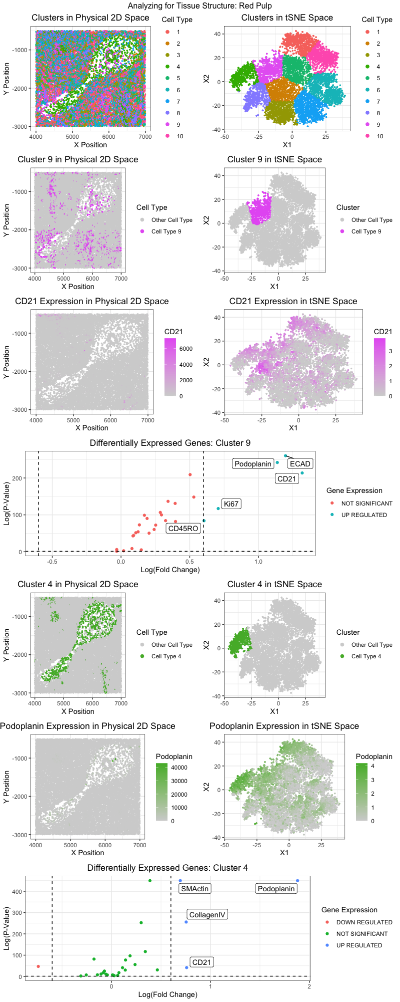
Figure Description:
Adapting the workflow from homework 5 (k-means clustering and differential gene expression analysis), I believe I was able to identify two distinct cell types in clusters 9 and cluster 4. I first utilized tSNE to reduce the dimensionality of the data and utilized the elbow-method to determine the optimal number of clusters to run the k-means clustering algorithm on. The identified clusters can both be visualized in physical 2D space and the reduced tSNE space.
For cluster 9, which preferentially expressed Ki67, Podoplanin, CD21, and CD45RO, I believe the cluster is composed of lymphocytes. Such differentially expressed genes can be seen in the volcano plot for cluster 9 Ki67 is not a distinct marker of any single cell type, but is rather a marker of proliferating cells [1]. Podoplanin is a marker often found in both adaptive and innate immune cells (both phagocytes and lymphocytes) [2]. CD21 is a known marker of mature B-cells, while CD45RO is a known marker of memory-T cells [3,4].
For cluster 4, which preferentially expressed SMActin, Podoplanin, and Collagen IV, I believe the cluster is composed of endothelial cells. SMActin (smooth muscle actin) is found in vessel endothelial cells [5]. CollagenIV is a vascular marker often found on the walls of vessels and arteries [6].
Hence, with the understanding that cluster 9 is composed of lymphocytes and cluster 4 is composed of endothelial cells (most likely forming the walls of a vessel or artery), I believe that the tissue structure captured in the CODEX dataset is that of Red Pulp. According to a paper, “the red pulp consists of venous sinuses filled with blood and cords of lymphatic cells, such as lymphocytes and macrophages” [7]. Venous sinuses are composed of endothelial cells, and lymphocytes were identified to be present in cluster 9. The spleen is composed of multiple tissue spaces that help transport immune cells throughout our body. Being a key component of the lymphatic system, I believe the CODEX dataset captures the protein expression of lymphocytes in the act of being transported to other areas of the body.
References:
[1] 10.1007/s00412-018-0659-8
[2] 10.2147/JIR.S366620
[3] 10.4049/jimmunol.167.1.163
[4] 10.7860/JCDR/2017/26866.9930
[5] 10.3960/jslrt.19032
[6] 10.3389/fimmu.2020.616531
[7] 10.1080/01926230600867743
## Load the necessary packages
library(ggplot2)
library(gridExtra)
library(ggrepel)
library(factoextra)
library(NbClust)
library(cluster)
library(Rtsne)
library(patchwork)

## Load the data
data <- read.csv('codex_spleen_subset.csv.gz', row.names = 1)

## Isolate columns of interest
pos <- data[,1:2]
area <- data[,3]
gexp <- data[,4:31]

## Isolate cells that have gene Expression
good_cells <- rownames(gexp)[rowSums(gexp) > 0]
pos <- pos[good_cells,]
gexp <- gexp[good_cells,]

## Normalize the data
tot_gexp <- rowSums(gexp)
norm_gexp <- gexp/tot_gexp * median(tot_gexp)
log_norm_gexp <- log10(norm_gexp + 1)

## Set seed for reproducibility
set.seed(1)

## Run tSNE analysis
emb <- Rtsne(log_norm_gexp, check = F)

## Determine the optimal number of k's (centroids) for kMeans
withinnes_list <- sapply(c(5:20), function(k) {
  tmp = kmeans(emb$Y, centers = k)
  return(tmp$tot.withinss)} )

elbow <- ggplot(data.frame(k = c(5:20), tot_withinss = withinnes_list), aes(k, tot_withinss)) +
  geom_point()

elbow

## Identifying optimal number of k's
optimal_k <- 10

## Run kMeans
set.seed(1)
cluster_tSNE <- kmeans(emb$Y, centers = optimal_k)
df_cluster <- data.frame(pos, cell_type = as.factor(cluster_tSNE$cluster), log_norm_gexp, emb$Y)

## Visualizing cells in the 2D space
clusters_2D <- ggplot(data = df_cluster, aes(x = x, y = y, col = cell_type)) +
  geom_point(size = 0.5) +
  theme_bw() +
  theme(plot.title = element_text(hjust = 0.5)) +
  xlab("X Position") + ylab("Y Position") +
  guides(color = guide_legend(override.aes = list(size = 2))) +
  labs(title = 'Clusters in Physical 2D Space', col = "Cell Type")

clusters_2D

## Visualizing cells in the tSNE space
clusters_tSNE <- ggplot(data = df_cluster, aes(x = X1, y = X2, col = cell_type)) +
  geom_point(size = 0.5) +
  theme_bw() +
  theme(plot.title = element_text(hjust = 0.5)) +
  guides(color = guide_legend(override.aes = list(size = 2))) +
  labs(title = 'Clusters in tSNE Space', col = "Cell Type")

clusters_tSNE

#############################################################################

## Picking a cluster (cluster 9)

## Visualizing Cluster 9 in Physical 2D Space
cluster9_2D <- ggplot(data = df_cluster, aes(x = x, y = y, col = cell_type == 9)) +
  geom_point(size = 0.5) +
  theme_bw() +
  theme(plot.title = element_text(hjust = 0.5)) +
  guides(color = guide_legend(override.aes = list(size = 2))) +
  labs(title = 'Cluster 9 in Physical 2D Space') +
  xlab("X Position") + ylab("Y Position") +
  scale_color_manual(name = 'Cell Type',
                     values = c('lightgrey', '#E665F3'),
                     labels = c('Other Cell Type', 'Cell Type 9'))

cluster9_2D

## Visualizing Cluster 9 in the tSNE Space
cluster9_tSNE <- ggplot(data = df_cluster, aes(x = X1, y = X2, col = cell_type == 9)) +
  geom_point(size = 0.5) +
  theme_bw() +
  theme(plot.title = element_text(hjust = 0.5)) +
  guides(color = guide_legend(override.aes = list(size = 2))) +
  labs(title = 'Cluster 9 in tSNE Space') +
  scale_color_manual(name = 'Cluster',
                     values = c('lightgrey', '#E665F3'),
                     labels = c('Other Cell Type', 'Cell Type 9'))

cluster9_tSNE

## Distinguishing between cells that are & are not within Cluster 9
cluster9 <- df_cluster[df_cluster$cell_type == 9, ]
not_cluster9 <- df_cluster[df_cluster$cell_type != 9, ]

## Identifying differentially expressed genes w/in Cluster 9 w/ Wilcox Rank Test
interest_genes <- sapply(colnames(log_norm_gexp), function(g){
  wilcox.test(log_norm_gexp[row.names(cluster9), g],
              log_norm_gexp[row.names(not_cluster9), g])$p.value
})

## Calculating log(fold_change) for Cluster 9 --> to generate volcano plot
log_fc <- sapply(colnames(log_norm_gexp), function(g) {
  log2( mean(log_norm_gexp[row.names(cluster9), g])
        / mean(log_norm_gexp[row.names(not_cluster9), g])) ## do ratio (log_2(A/B))
})

volcano_9 <- data.frame(log_fc, log_p_val = ifelse(is.infinite(-log10(interest_genes)), 350, -log10(interest_genes)))

genes_upregulated_9 <- sapply(colnames(log_norm_gexp), function(g){
  wilcox.test(log_norm_gexp[row.names(cluster9), g],
              log_norm_gexp[row.names(not_cluster9), g],
              alternative = 'greater')$p.value
})

top_10_gene_9 <- names(which(genes_upregulated_9 < 0.05 & log_fc > 0.6))
top_10_gene_9 <- genes_upregulated_9[top_10_gene_9]
top_10_gene_9 ## top 10 are Ki67, Podoplanin, CD21, CD45RO, and ECAD

## For coloring in the points for volcano plot
volcano_9$diff_express <- "NOT SIGNIFICANT"
volcano_9$diff_express[volcano_9$log_fc > 0.6 & volcano_9$log_p_val > -log10(0.05)] <- "UP REGULATED"
volcano_9$diff_express[volcano_9$log_fc < -0.6 & volcano_9$log_p_val > -log10(0.05)] <- "DOWN REGULATED"

## Creating volcano plot to visualize upregulated genes in Cluster 9!
volcano_plot_9 <- ggplot(volcano_9) +
  geom_point(aes(x = log_fc, y = log_p_val, col = diff_express)) +
  geom_vline(xintercept = c(-0.6, 0.6), linetype = 'dashed') +
  geom_hline(yintercept=-log10(0.05), linetype = 'dashed') +
  geom_label_repel(data = volcano_9[names(top_10_gene_9),],
                   aes(x = log_fc, y = log_p_val, label = names(top_10_gene_9)),
                   max.overlaps = 40) +
  theme_bw() +
  labs(title = 'Differentially Expressed Genes: Cluster 9',
       x = 'Log(Fold Change)', y = 'Log(P-Value)', col = "Gene Expression") +
  theme(plot.title = element_text(hjust = 0.5))

volcano_plot_9

## Plot the top most significant genes (CD21)

## Plotting in Physical 2D Space
gene9_2d <- ggplot(data = data, aes(x = x, y = y, col = CD21)) +
  geom_point(size = 0.5) +
  theme_bw() +
  scale_color_gradient(low = 'lightgrey', high = '#E665F3') +
  labs(x = "X Position", y = "Y Position", color = "CD21", title = "CD21 Expression in Physical 2D Space") +
  theme(plot.title = element_text(hjust = 0.5))

gene9_2d

## Plotting in tSNE Space
gene9_tSNE <- ggplot(data = df_cluster, aes(x = X1, y = X2, col = CD21)) +
  geom_point(size = 0.5) +
  theme_bw() +
  scale_color_gradient(low = 'lightgrey', high = '#E665F3') +
  labs(color = "CD21", title = "CD21 Expression in tSNE Space") +
  theme(plot.title = element_text(hjust = 0.5))

gene9_tSNE

#############################################################################

## Picking another cluster (cluster 4)

## Visualizing Cluster 4 in Physical 2D Space
cluster4_2D <- ggplot(data = df_cluster, aes(x = x, y = y, col = cell_type == 4)) +
  geom_point(size = 0.5) +
  theme_bw() +
  theme(plot.title = element_text(hjust = 0.5)) +
  guides(color = guide_legend(override.aes = list(size = 2))) +
  labs(title = 'Cluster 4 in Physical 2D Space') +
  xlab("X Position") + ylab("Y Position") +
  scale_color_manual(name = 'Cell Type',
                     values = c('lightgrey', '#53B535'),
                     labels = c('Other Cell Type', 'Cell Type 4'))

cluster4_2D

## Visualizing Cluster 4 in the tSNE Space
cluster4_tSNE <- ggplot(data = df_cluster, aes(x = X1, y = X2, col = cell_type == 4)) +
  geom_point(size = 0.5) +
  theme_bw() +
  theme(plot.title = element_text(hjust = 0.5)) +
  guides(color = guide_legend(override.aes = list(size = 2))) +
  labs(title = 'Cluster 4 in tSNE Space') +
  scale_color_manual(name = 'Cluster',
                     values = c('lightgrey', '#53B535'),
                     labels = c('Other Cell Type', 'Cell Type 4'))

cluster4_tSNE

## Distinguishing between cells that are & are not within Cluster 4
cluster4 <- df_cluster[df_cluster$cell_type == 4, ]
not_cluster4 <- df_cluster[df_cluster$cell_type != 4, ]

## Identifying differentially expressed genes w/in Cluster 4 w/ Wilcox Rank Test
interest_genes <- sapply(colnames(log_norm_gexp), function(g){
  wilcox.test(log_norm_gexp[row.names(cluster4), g],
              log_norm_gexp[row.names(not_cluster4), g])$p.value
})

## Calculating log(fold_change) for Cluster 4 --> to generate volcano plot
log_fc <- sapply(colnames(log_norm_gexp), function(g) {
  log2( mean(log_norm_gexp[row.names(cluster4), g])
        / mean(log_norm_gexp[row.names(not_cluster4), g])) ## do ratio (log_2(A/B))
})

volcano_4 <- data.frame(log_fc, log_p_val = ifelse(is.infinite(-log10(interest_genes)), 450, -log10(interest_genes)))

genes_upregulated_4 <- sapply(colnames(log_norm_gexp), function(g){
  wilcox.test(log_norm_gexp[row.names(cluster4), g],
              log_norm_gexp[row.names(not_cluster4), g],
              alternative = 'greater')$p.value
})

top_10_gene_4 <- names(which(genes_upregulated_4 < 0.05 & log_fc > 0.6))
top_10_gene_4 <- genes_upregulated_4[top_10_gene_4]
top_10_gene_4 ## top 10 are SMActin, Podoplanin, CD21, CollagenIV

## For coloring in the points for volcano plot
volcano_4$diff_express <- "NOT SIGNIFICANT"
volcano_4$diff_express[volcano_4$log_fc > 0.6 & volcano_4$log_p_val > -log10(0.05)] <- "UP REGULATED"
volcano_4$diff_express[volcano_4$log_fc < -0.6 & volcano_4$log_p_val > -log10(0.05)] <- "DOWN REGULATED"

## Creating volcano_4 plot to visualize upregulated genes in Cluster 4!
volcano_plot_4 <- ggplot(volcano_4) +
  geom_point(aes(x = log_fc, y = log_p_val, col = diff_express)) +
  geom_vline(xintercept = c(-0.6, 0.6), linetype = 'dashed') +
  geom_hline(yintercept=-log10(0.05), linetype = 'dashed') +
  geom_label_repel(data = volcano_4[names(top_10_gene_4),],
                   aes(x = log_fc, y = log_p_val, label = names(top_10_gene_4)),
                   max.overlaps = 40) +
  theme_bw() +
  labs(title = 'Differentially Expressed Genes: Cluster 4',
       x = 'Log(Fold Change)', y = 'Log(P-Value)', col = "Gene Expression") +
  theme(plot.title = element_text(hjust = 0.5))

volcano_plot_4

## Plot the top most significant genes (Podoplanin)

## Plotting in Physical 2D Space
gene4_2d <- ggplot(data = data, aes(x = x, y = y, col = Podoplanin)) +
  geom_point(size = 0.5) +
  theme_bw() +
  scale_color_gradient(low = 'lightgrey', high = '#53B535') +
  labs(x = "X Position", y = "Y Position", color = "Podoplanin", title = "Podoplanin Expression in Physical 2D Space") +
  theme(plot.title = element_text(hjust = 0.5))

gene4_2d

## Plotting in tSNE Space
gene4_tSNE <- ggplot(data = df_cluster, aes(x = X1, y = X2, col = Podoplanin)) +
  geom_point(size = 0.5) +
  theme_bw() +
  scale_color_gradient(low = 'lightgrey', high = '#53B535') +
  labs(color = "Podoplanin", title = "Podoplanin Expression in tSNE Space") +
  theme(plot.title = element_text(hjust = 0.5))

gene4_tSNE

#############################################################################

## Combining all the plots together
lay <- rbind(c(1,2),
             c(3,4),
             c(5,6),
             c(7,7),
             c(8,9),
             c(10,11),
             c(12,12))

grid.arrange(clusters_2D, clusters_tSNE,
             cluster9_2D, cluster9_tSNE,
             gene9_2d, gene9_tSNE,
             volcano_plot_9,
             cluster4_2D, cluster4_tSNE,
             gene4_2d, gene4_tSNE,
             volcano_plot_4,
             layout_matrix = lay,
             top = "Analyzing for Tissue Structure: Red Pulp") # width 800, height 2000

## References:
## (1) To determine the optimal number of clusters
## https://medium.com/@chyun55555/how-to-find-the-optimal-number-of-clusters-with-r-dbf84588388b
## (2) Graphing volcano plots
## https://biocorecrg.github.io/CRG_RIntroduction/volcano-plots.html