CODEX Data Exploration and Analysis of the Spleen

Description of Visualization

Here is a brief description of each plot in the visualization:

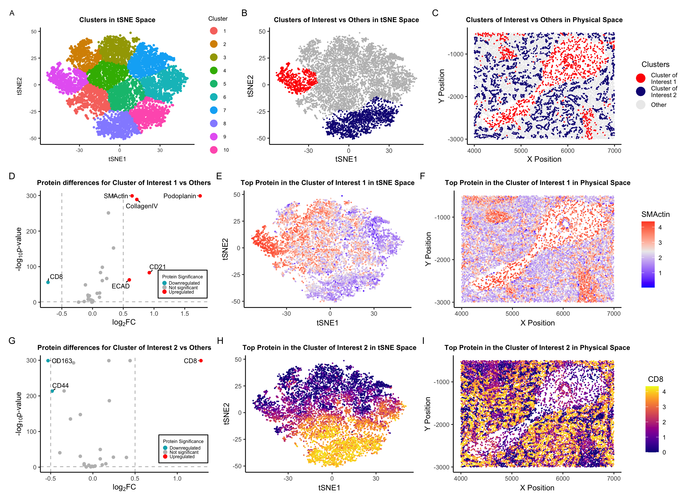
A. Clusters in t-SNE Space: A t-SNE (t-distributed Stochastic Neighbor Embedding) plot showing clusters of data points representing protein expression within the CODEX data. Different colors represent distinct clusters, labeled from 1 to 10.

B. Clusters of Interest vs Others in t-SNE Space: Another t-SNE plot focusing on two clusters of interest, colored in red and blue, while other data points are in gray. This highlights the distribution and separation of these two clusters from the rest. NOTE: I combined clusters 8 and 9 into one cluster (Cluster of Interest 2) for downstream analysis.

C. Clusters of Interest vs Others in Physical Space: This plot shows the spatial distribution of the clusters of interest versus others in the physical space.

D. Protein differences for Cluster of Interest 1 vs Others: A volcano plot displaying the log2 fold change (log2FC) on the x-axis against the negative logarithm of the p-value (-log10 p-value) on the y-axis. Points represent individual proteins, with their significance indicated by color: red for upregulated, gray for not significant, and blue for downregulated. Notable proteins are labeled, such as “SMActin,” “Podoplanin,” “CollagenIV,” “CD21,” “CD8,” and “ECAD.”

E. Top Protein in the Cluster of Interest 1 in t-SNE Space: A t-SNE plot colored by the expression level of a top protein, SMActin, in Cluster of Interest 1, with a gradient color (blue-white-red) scale indicating low to high expression levels.

F. Top Protein in the Cluster of Interest 1 in Physical Space: Similar to panel C, this plot shows the physical distribution of SMActin expression level in Cluster of Interest 1, with the same color gradient as panel E.

G. Protein differences for Cluster of Interest 2 vs Others: Another volcano plot like in panel D, but for Cluster of Interest 2. The data points are colored by their significance in relation to protein expression, with notable proteins labeled, such as “CD8” and “CD163.”

H. Top Protein in the Cluster of Interest 2 in t-SNE Space: A t-SNE plot that visualizes the expression level of a top protein, CD8, in Cluster of Interest 2, with the viridis-plasma gradient.

I. Top Protein in the Cluster of Interest 2 in Physical Space: This plot shows the physical space distribution of CD8 in Cluster of Interest 2, using the viridis-plasma color gradient to represent expression levels.

Cell Type Interpretation for Clusters

Cluster of Interest 1 has multiple proteins that are highly expressed, including SMActin, Podoplanin, CollagenIV, CD21, and ECAD. SMActin is a protein that is highly expressed in smooth muscle cells and is involved in cell motility and contraction [1]. Podoplanin is a protein that is highly expressed in lymphatic endothelial cells and is involved in cell migration and adhesion [2]. CollagenIV is a protein that is highly expressed in the basement membrane and is involved in cell adhesion and migration [3]. Therefore, with this in mind I would guess that Cluster of Interest 1 is likely composed of smooth muscle cells and lymphatic endothelial cells.

Cluster of Interest 2 is likely composed of T cells, as it is highly enriched for the CD8 protein which are known to be expressed in T cells [4]. However, this cluster is likely not solely composed of T-cells as the next highly expressed protein is Lyve1 which is known to be expressed on the lymphatic endothelial cells and acts as a hyaluronan transport [5].

Tissue Structure Guess

Based on my results, I would guess this tissue contains at least Artery/Vein and White pulp. This is because the proteins expressed in the clusters of interest are known to be expressed in these tissues. For example, Lyve1 is known to be expressed in lymphatic vessels and CD8 is known to be expressed in white pulp [6]. However, I didn’t explore the other clusters in detail, so it is possible that other tissues are present as well!

References

[1] https://www.sciencedirect.com/topics/medicine-and-dentistry/smooth-muscle-actin

[2] https://www.ncbi.nlm.nih.gov/pmc/articles/PMC5980289/#:~:text=Podoplanin%20(PDPN)%20is%20a%20unique,of%20approximately%2010%20amino%20acids.

[3] https://www.ncbi.nlm.nih.gov/gene/1282

[4] https://www.ncbi.nlm.nih.gov/gene/925

[5] https://www.rndsystems.com/resources/articles/lyve-1-functions-use-lymphatic-marker

[6] https://www.sciencedirect.com/topics/veterinary-science-and-veterinary-medicine/white-pulp#:~:text=White%20pulp%20is%20composed%20of,structural%20framework%20of%20the%20spleen.

Note: I decided to use viridis-plasma for the color scale in some plots based on other students figures (I think it looks good)! The rest of the code is reused from my previous homeworks with some additions.

Code

### HW6 ###
## Caleb Hallinan ##
## Pikachu sequencing data ##

# import libraries
library(here)
library(ggplot2)
library(Rtsne)
library(patchwork)
library(factoextra)
library(ggrepel)
library(viridis)

# set seed
set.seed(02052024)


#### Data Preprocessing ####

# read in data
data <- read.csv('~/Desktop/jhu/classes/genomic-data-visualization-2024/data/codex_spleen_subset.csv.gz', row.names=1)
head(data)
dim(data)

# extract data
pos <- data[, 1:2]
area <- data[, 3]
pexp <- data[, 4:31]
head(pexp)

# normalize
pexpnorm <- log10(pexp/rowSums(pexp) * mean(rowSums(pexp))+1)
head(pexpnorm)


#### Dimensionality Reduction ####

# perform pca
pcs <- prcomp(pexpnorm)

# run tsne on top PCs
set.seed(02052024)
emb <- Rtsne(pexpnorm, perplexity = 15) # can change dims from 
# names(emb)


#### Clustering ####

#create plot of number of clusters vs total within sum of squares
# fviz_nbclust(data.frame(emb$Y), kmeans, method = "wss")

# perform kemans clustering based on elbow plot
set.seed(02052024)
clusters <- as.factor(kmeans(emb$Y, 10)$cluster)
# cluster of interest
int_clus <- 9
int_clus2 <- c(8,10)

# get just cluster of interest
cluster_of_interest <- ifelse(clusters == int_clus, "Cluster of\nInterest 1", "Other")
cluster_of_interest <- ifelse(clusters %in% int_clus2, "Cluster of\nInterest 2", cluster_of_interest)


# plot tsne to see
clus_plt <- ggplot(data.frame(emb$Y)) +
  geom_point(aes(x = emb$Y[,1], y = emb$Y[,2], color = clusters), size=0.75) +
  theme_classic() +
  labs(
    title = "Clusters in tSNE Space",
    color = "Cluster",
    x = "tSNE1",
    y = "tSNE2"
  ) +
  theme(legend.title.align=0.5,plot.title = element_text(hjust = 0.5, face="bold", size=9), text = element_text(size = 8)) +
  guides(color = guide_legend(override.aes = list(size=4)))


#### DE Protein Analysis ####

# do wilcox for DE protein analysis
pv <- sapply(colnames(pexpnorm), function(i) {
  print(i) ## print out gene name
  wilcox.test(pexpnorm[clusters == int_clus, i], pexpnorm[clusters != int_clus, i])$p.val
})

head(sort(pv))

# get log fold change
logfc <- sapply(colnames(pexpnorm), function(i) {
  print(i) ## print out gene name
  log2(mean(pexpnorm[clusters == int_clus, i])/mean(pexpnorm[clusters != int_clus, i]))
})


# do wilcox for DE protein analysis
pv_2 <- sapply(colnames(pexpnorm), function(i) {
  print(i) ## print out gene name
  wilcox.test(pexpnorm[clusters %in% int_clus2, i], pexpnorm[!clusters %in% int_clus2, i])$p.val
})

head(sort(pv_2))

# get log fold change
logfc_2 <- sapply(colnames(pexpnorm), function(i) {
  print(i) ## print out gene name
  log2(mean(pexpnorm[clusters %in% int_clus2, i])/mean(pexpnorm[!clusters %in% int_clus2, i]))
})

### Plotting ###

# protein to plot
gene <- names(sort(pv)[1])
gene_2 <- names(sort(pv_2)[1])

# add cluster of interest to data
data$cluster_of_interest <- cluster_of_interest
# add gene of interest to data
data$gene_of_interest <- pexpnorm[[gene]]
data$gene_of_interest_2 <- pexpnorm[[gene_2]]

# create df for tsne to plot layers
tsne_emb <- data.frame(emb$Y)
tsne_emb$cluster_of_interest <- cluster_of_interest
tsne_emb$gene_of_interest <- pexpnorm[[gene]]
tsne_emb$gene_of_interest_2 <- pexpnorm[[gene_2]]


top1 <- ggplot(data.frame(emb$Y)) +
  geom_point(aes(x = emb$Y[,1], y = emb$Y[,2], color = cluster_of_interest), size=0.2) +
  scale_color_manual(values = c("red", "#151784","gray")) +
  theme_classic() +
  labs(
    title = "Clusters of Interest vs Others in tSNE Space",
    color = "Clusters",
    x = "tSNE1",
    y = "tSNE2"
  ) +
  # scale_color_gradient2(midpoint = median(pexpnorm[[gene]]), low = "blue", mid = "#ECECEC", high = "red", space = "Lab" ) +
  theme(legend.title.align=0.5,plot.title = element_text(hjust = 0.5, face="bold", size=9), text = element_text(size = 10)) +
  guides(color = "none") 


top2 <- ggplot() +
  geom_point(data = data[cluster_of_interest == "Other",], aes(x = x, y = y, color = cluster_of_interest), size=0.01) +
  geom_point(data = data[cluster_of_interest == "Cluster of\nInterest 1",], aes(x = x, y = y, color = cluster_of_interest), size=0.2) +
  geom_point(data = data[cluster_of_interest == "Cluster of\nInterest 2",], aes(x = x, y = y, color = cluster_of_interest), size=0.2) +
  scale_color_manual(values = c("red","#151784","#ECECEC")) +
  # scale_color_gradient2(midpoint = max(pexpnorm[[gene]])/2, low = "blue", mid = "#ECECEC", high = "red", space = "Lab" ) +
  theme_classic() +
  labs(
    title = "Clusters of Interest vs Others in Physical Space",
    color = "Clusters",
    x = "X Position",
    y = "Y Position"
  ) +
  guides(size = "none",color = guide_legend(override.aes = list(size=5))) + 
  theme(legend.title.align=0.5, plot.title = element_text(hjust = 0.5, face="bold", size=9), 
        text = element_text(size = 10))

# plot tsne to see
bottom1 <-ggplot(tsne_emb) +
  geom_point(data = tsne_emb[cluster_of_interest == "Other",], aes(x = X1, y = X2, color = gene_of_interest), size=0.2) +
  geom_point(data = tsne_emb[cluster_of_interest == "Cluster of\nInterest 2",], aes(x = X1, y = X2, color = gene_of_interest), size=0.2) +
  geom_point(data = tsne_emb[cluster_of_interest == "Cluster of\nInterest 1",], aes(x = X1, y = X2, color = gene_of_interest), size=0.2) +
  theme_classic() +
  labs(
    title = "Top Protein in the Cluster of Interest 1 in tSNE Space",
    color = gene,
    x = "tSNE1",
    y = "tSNE2"
  ) +
  scale_color_gradient2(midpoint = median(pexpnorm[[gene]]), low = "blue", mid = "#ECECEC", high = "red", space = "Lab" ) +
  # scale_color_gradient(low = "#ECECEC", high = "red", space = "Lab" ) +
  theme(legend.title.align=0.5,plot.title = element_text(hjust = 0.5, face="bold", size=9), text = element_text(size = 10)) +
  guides(color = "none")



bottom2 <- ggplot(data) +
  geom_point(data = data[cluster_of_interest == "Other",], aes(x = x, y = y, color = gene_of_interest[cluster_of_interest == "Other"]), size=0.2) +
  geom_point(data = data[cluster_of_interest == "Cluster of\nInterest 2",], aes(x = x, y = y, color = gene_of_interest[cluster_of_interest == "Cluster of\nInterest 2"]), size=0.2) +
  geom_point(data = data[cluster_of_interest == "Cluster of\nInterest 1",], aes(x = x, y = y, color = gene_of_interest[cluster_of_interest == "Cluster of\nInterest 1"]), size=0.2) +
  # scale_color_gradient(low = "#ECECEC", high = "red", space = "Lab" ) +
  scale_color_gradient2(midpoint = median(pexpnorm[[gene]]), low = "blue", mid = "#ECECEC", high = "red", space = "Lab" ) +
  theme_classic() +
  labs(
    title = "Top Protein in the Cluster of Interest 1 in Physical Space",
    color = gene,
    x = "X Position",
    y = "Y Position"
  ) +
  guides(size = "none") + 
  theme(legend.title.align=0.5,plot.title = element_text(hjust = 0.5, face="bold", size=9), 
        text = element_text(size = 10))


# plot tsne to see
bottom1_2 <- ggplot(tsne_emb) +
  geom_point(data = tsne_emb[cluster_of_interest == "Other",], aes(x = X1, y = X2, color = gene_of_interest_2), size=0.2) +
  geom_point(data = tsne_emb[cluster_of_interest == "Cluster of\nInterest 1",], aes(x = X1, y = X2, color = gene_of_interest_2), size=0.2) +
  geom_point(data = tsne_emb[cluster_of_interest == "Cluster of\nInterest 2",], aes(x = X1, y = X2, color = gene_of_interest_2), size=0.2) +
  theme_classic() +
  labs(
    title = "Top Protein in the Cluster of Interest 2 in tSNE Space",
    color = gene_2,
    x = "tSNE1",
    y = "tSNE2"
  ) +
  theme(legend.title.align=0.5,plot.title = element_text(hjust = 0.5, face="bold", size=9), text = element_text(size = 10)) +
  guides(color = "none")+ 
  scale_color_viridis(option="plasma")


bottom2_2 <- ggplot(data) +
  geom_point(data = data[cluster_of_interest == "Other",], aes(x = x, y = y, color = gene_of_interest_2[cluster_of_interest == "Other"]), size=0.2) +
  geom_point(data = data[cluster_of_interest == "Cluster of\nInterest 1",], aes(x = x, y = y, color = gene_of_interest_2[cluster_of_interest == "Cluster of\nInterest 1"]), size=0.2) +
  geom_point(data = data[cluster_of_interest == "Cluster of\nInterest 2",], aes(x = x, y = y, color = gene_of_interest_2[cluster_of_interest == "Cluster of\nInterest 2"]), size=0.2) +
  theme_classic() +
  labs(
    title = "Top Protein in the Cluster of Interest 2 in Physical Space",
    color = gene_2,
    x = "X Position",
    y = "Y Position"
  ) +
  guides(size = "none") + 
  theme(legend.title.align=0.5,plot.title = element_text(hjust = 0.5, face="bold", size=9), 
        text = element_text(size = 10)) + 
  scale_color_viridis(option="plasma")


# volcano plot
df <- data.frame(pv=-log10(pv + 10e-300), logfc)
# add gene names
df$genes <- rownames(df)
# add labeling
df$delabel <- ifelse(df$logfc > 0.5, df$genes, NA)
df$delabel <- ifelse(df$logfc < -0.5, df$genes, df$delabel)
# add if DE 
df$diffexpressed <- ifelse(df$logfc > 0.5, "Upregulated", "Not Significant")
df$diffexpressed <- ifelse(df$logfc < -0.5, "Downregulated", df$diffexpressed)

# plot
mid <- ggplot(df, aes(x = logfc, y = pv, label = delabel, color = diffexpressed)) + 
  geom_point(size= 1.5) +
  geom_vline(xintercept = c(-0.5, 0.5), col = "gray", linetype = 'dashed') +
  geom_hline(yintercept = -log10(0.05), col = "gray", linetype = 'dashed') +
  scale_color_manual(values = c("#00AFBB", "grey", "red"),
                     labels = c("Downregulated", "Not significant", "Upregulated")) +
  # theme
  theme_classic() +
  # labels
  labs(color = 'Protein Significance', 
       x = expression("log"[2]*"FC"), 
       y = expression("-log"[10]*"p-value"),
       title = "Protein differences for Cluster of Interest 1 vs Others") +
  theme(
    plot.title = element_text(hjust = 0.5, face="bold", size=9),
    text = element_text(size = 10),
    legend.position = c(0.85, 0.2), # Adjust these values to move the legend inside the plot
    legend.background = element_rect(fill = "white", colour = "black"),
    legend.text = element_text(size = 6), # Makes legend text smaller
    legend.title = element_text(size = 6), # Makes legend title smaller
    legend.key.size = unit(0.15, "cm") # Makes the legend keys smaller
  ) + 
  geom_text_repel(max.overlaps = Inf, box.padding = 0.25, point.padding = 0.25, min.segment.length = 0, size = 3, color = "black") + 
  scale_x_continuous(breaks = seq(-5, 5, 0.5)) +
  guides(size = "none",color = guide_legend(override.aes = list(size=2)))


# volcano plot
df <- data.frame(pv_2=-log10(pv_2 + 10e-300), logfc_2)
# add gene names
df$genes <- rownames(df)
# add labeling
df$delabel <- ifelse(df$logfc > 0.5, df$genes, NA)
df$delabel <- ifelse(df$logfc < -0.45, df$genes, df$delabel)
# add if DE 
df$diffexpressed <- ifelse(df$logfc > 0.5, "Upregulated", "Not Significant")
df$diffexpressed <- ifelse(df$logfc < -0.45, "Downregulated", df$diffexpressed)

# plot
mid_2 <- ggplot(df, aes(x = logfc_2, y = pv_2, label = delabel, color = diffexpressed)) + 
  geom_point(size= 1.5) +
  geom_vline(xintercept = c(-0.5, 0.5), col = "gray", linetype = 'dashed') +
  geom_hline(yintercept = -log10(0.05), col = "gray", linetype = 'dashed') +
  scale_color_manual(values = c("#00AFBB", "grey", "red"),
                     labels = c("Downregulated", "Not significant", "Upregulated")) +
  # theme
  theme_classic() +
  # labels
  labs(color = 'Protein Significance', 
       x = expression("log"[2]*"FC"), 
       y = expression("-log"[10]*"p-value"),
       title = "Protein differences for Cluster of Interest 2 vs Others") +
  theme(
    plot.title = element_text(hjust = 0.5, face="bold", size=9),
    text = element_text(size = 10),
    legend.position = c(0.85, 0.2), # Adjust these values to move the legend inside the plot
    legend.background = element_rect(fill = "white", colour = "black"),
    legend.text = element_text(size = 6), # Makes legend text smaller
    legend.title = element_text(size = 6), # Makes legend title smaller
    legend.key.size = unit(0.15, "cm") # Makes the legend keys smaller
  ) + 
  geom_text_repel(max.overlaps = Inf, box.padding = 0.25, point.padding = 0.25, min.segment.length = 0, size = 3, color = "black") + 
  scale_x_continuous(breaks = seq(-5, 5, 0.5)) +
  guides(size = "none", color = guide_legend(override.aes = list(size=2)))


# plot using patchwork
(clus_plt + top1 + top2) / (mid + bottom1 + bottom2) / (mid_2 + bottom1_2 + bottom2_2) + plot_annotation(tag_levels = 'A')