Identification of White Pulp Tissue Through K-Means Analysis of CORDEX Data

What am I visualizing?
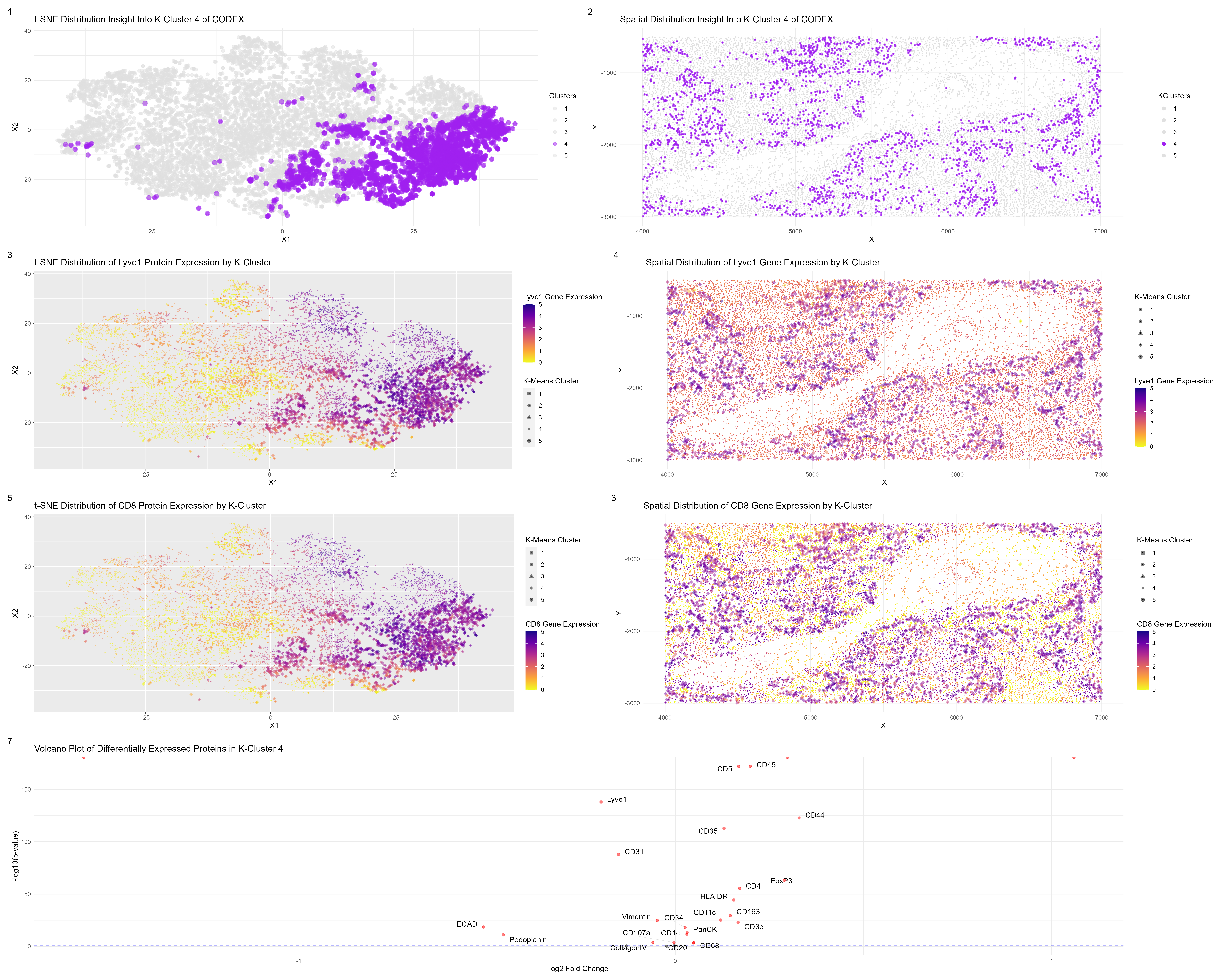
Here, I am visualizing a particular cluster from the CORDEX dataset, full of proteins, of an unknown tissue structure, in the hope of identifying the tissue by identifying several cell-types. In my particular cluster of interest (cluster 4), I noticed that immune cells and markers for immune cells were differentially expressed and upregulated. I decided to visualize the expression of two of these differentially expressed proteins, CD8 and Lyve1.
Subplot 1 displays the t-SNE distribution of my partial components and highlights my chosen cluster, while subplot 2 displays the spatial distribution of my cluster of interest.
Subplot 3 displays the t-SNE distribution of my partial components but highlights the expression level of my gene of interest, CD8, throughout the tissue as well as displaying the k-means clusters. Subplot 4 also displays a similar visual but uses spatial distribution in the physical space of the tissue instead. Note that in both visuals, cluster 4 is highlighted (hence a bigger point shape) and has very high expression levels of Lyve1. From my research, Lyve1 is a common marker for lymphatic endothelial cells (LEC) [1], and in one paper was mainly observed in sinusoidal-like networks surrounding the lymphocyte-rich white pulp in the spleen [1]. Therefore this cluster has LECs.
Subplot 5 displays the t-SNE distribution of my partial components but highlights the expression level of my gene of interest, CD8, throughout the tissue as well as displaying the k-means clusters. Subplot 6 also displays a similar visual but uses spatial distribution in the physical space of the tissue instead. In both visuals, cluster 4 is once again highlighted (hence a bigger point shape) and has very high expression levels of CD8. CD8 is a type of T-cell that plays an important role in immune response. From my research, the spleen is the most important priming site for generating CD8 T cell immunity [2]. In one paper, CD8α+ dendritic cells attach to bacteria and transport and then move to the white pulp of the spleen where CD8 T cells can begin an immune response against bacteria [2]. This gives more reasoning that we are in the spleen and in the white pulp of the spleen and how we have T-cells and other immune cells in this cluster.
Subplot 7 is a volcano plot of my differentially expressed genes in my chosen cluster, showing what proteins are upregulated or underregulated.
What was your process? Why do I believe I identified the same cell-types?
I looked at several clusters and performed a Wilicox ranked sum test to see what proteins were differentially expressed and upregulated, and noted that some of the top DE proteins were common immune markers/cells. I did a quick consult with ChatGBT, and noted that CD45RO was a marker for memory T cells, CD15 is typically expressed on granulocytes and some monocytes, CD45 is a common leukocyte antigen expressed on all hematopoietic cells, CD5 is a marker for T cells and a subset of B cells, CD44 is a cell adhesion molecule expressed on a variety of cells, including leukocytes, and CD35 is found on various immune cells, including B cells and dendritic cells. A lot of these clusters seem to be comprised of immune cell-types. I then read up on several papers to confirm this and saw that, for example, CD45RO was associated with T lymphocytes [3]. More and more research made me believe we were in the spleen and in particular, white pulp, because of the lymphoid tissue present and abundance of immune cells. White pulp generates a lot of antigen immune responses. I think chose to focus on cluster 4 and confirmed the top DE/upregulated proteins were in fact immune cells and then focused on CD8 andLyve1.
In the end, this tissue structure is white-pulp and has LECs and T-cells.
Resources
[1] Choi YK, Fallert Junecko BA, Klamar CR, Reinhart TA. Characterization of cells expressing lymphatic marker LYVE-1 in macaque large intestine during simian immunodeficiency virus infection identifies a large population of nonvascular LYVE-1(+)/DC-SIGN(+) cells. Lymphat Res Biol. 2013 Mar;11(1):26-34. doi: 10.1089/lrb.2012.0019. PMID: 23531182; PMCID: PMC3609640.
[2] Sharma N, Benechet AP, Lefrançois L, Khanna KM. CD8 T Cells Enter the Splenic T Cell Zones Independently of CCR7, but the Subsequent Expansion and Trafficking Patterns of Effector T Cells after Infection Are Dysregulated in the Absence of CCR7 Migratory Cues. J Immunol. 2015 Dec 1;195(11):5227-36. doi: 10.4049/jimmunol.1500993. Epub 2015 Oct 23. PMID: 26500349; PMCID: PMC4655190.
[3] Satoh T, Oikawa H, Yashima-Abo A, Nishiya M, Masuda T. Expression of mucosal addressin cell adhesion molecule-1 on the reticular framework between white pulp and the marginal zone in the human spleen. J Clin Exp Hematop. 2019;59(4):187-195. doi: 10.3960/jslrt.19032. PMID: 31866620; PMCID: PMC6954172.
[4] Bronte V, Pittet MJ. The spleen in local and systemic regulation of immunity. Immunity. 2013 Nov 14;39(5):806-18. doi: 10.1016/j.immuni.2013.10.010. Erratum in: Immunity. 2023 May 9;56(5):1152. PMID: 24238338; PMCID: PMC3912742.
# Dee Velazquez
# HW 5

#Get data
data <- read.csv("codex_spleen_subset.csv.gz", row.names = 1)

#Get dimns
dim(data)

#Get pos
pos <- data[1:2]

#Get area
area <-data[,3]

#Get protein expression
pexp <- data[,4:ncol(data)]

#Normalize protein expression
pexp_norm <- log10((pexp/area * mean(area))+1)

#PCA
pca <- prcomp(pexp_norm)
head(pca$x[,1:5])
head(pca$sdev)
head(pca$rotation[,1:5])
head(sort(pca$rotation[,1], decreasing=TRUE))
#CD44     CD163       CD4   SMActin    CD45RO      CD68
head(sort(pca$rotation[,2], decreasing=TRUE))
#CD8     CD45RO       Ki67       CD3e Podoplanin       CD44
df <- data.frame(pca$x, pexp_norm)
#Find optimal k clusters
plot(pca$sdev[1:31])
#Find optimal k clusters
plot(pca$sdev[1:30])
results <- sapply(seq(1, 20, by=1), function(i) {
  #print(i)
  com <- kmeans(pca$x[,1:20], centers=i)
  return(com$tot.withinss)
})
results
plot(results, type="l")
#From plotting tot.withinss, not really clear but say around 5 cell types
com <- kmeans(pca$x[,1:20], centers=5)
table(com$cluster)

com2 <- kmeans(pexp_norm, centers=5)
com2 <- as.factor(kmeans(pexp_norm, centers=5)$cluster)
table(com2)

df2 <- data.frame(pos, kmeans=as.factor(com$cluster))
head(df2)
p1 <- ggplot(df2) + geom_point(aes(x = x, y=y, col=kmeans),
                               size=.5, alpha=.5) + theme_minimal()
p1 + guides(color = guide_legend(override.aes = list(size = 2)))
df3 <- data.frame(pca$x[,1:20], Cluster=as.factor(com$cluster))
p2 <- ggplot(df3) + geom_point(aes(x = PC1, y=PC2, col=Cluster),
                               size=.5, alpha=.5) + theme_minimal()
p2 + guides(color = guide_legend(override.aes = list(size = 2)))

#tSNE
emb <- Rtsne(pca$x[,1:20])$Y
df4 <- data.frame(emb, Clusters=as.factor(com$cluster))
p3 <- ggplot(df4) + geom_point(aes(x = X1, y = X2, col=Clusters), size=.5, alpha=0.5) +
  theme_bw()
p3 + guides(color = guide_legend(override.aes = list(size = 2)))

###
###
#Exploratory analysis
#Want to focus on cluster 4 , see what differentially expressed proteins
results <- sapply(colnames(pexp_norm), function(g) {
  wilcox.test(pexp_norm[com2 == 4, g],
              pexp_norm[com2 != 4, g],
              alternative = "two.sided")$p.val
})
head(sort(results, decreasing=FALSE))
# CD8,            CD45RO,           CD15,       CD45,       CD5,          Lyve1
#0.000000e+00  0.000000e+00  0.000000e+00 7.659858e-173 9.935800e-1    1.164494e-138
#...immune cells, particularly T-cells and B-cells
#Now see what proteins are differentitally up-regulated in cluster 4
results2 <- sapply(colnames(pexp_norm), function(g) {
  wilcox.test(pexp_norm[com2 == 4, g],
              pexp_norm[com2 != 4, g],
              alternative = "greater")$p.val
})
head(sort(results2, decreasing=FALSE))
# CD45RO          CD15          CD45           CD5          CD44        CD35
#0.000000e+00  0.000000e+00 3.829929e-173 4.967900e-173 9.206565e-124   5.501252e-114
#more various immune cells, particularly T-cells and B-cells.
#Want to focus on cluster 1 , see what differentially expressed proteins
results3 <- sapply(colnames(pexp_norm), function(g) {
  wilcox.test(pexp_norm[com2 == 1, g],
              pexp_norm[com2 != 1, g],
              alternative = "two.sided")$p.val
})
head(sort(results3, decreasing=FALSE))
#Ki67    Podoplanin          CD21          ECAD         FoxP3      `   CD45RO
#0.000000e+00  0.000000e+00  0.000000e+00  0.000000e+00  0.000000e+00 2.368812e-189
#Ki67 is often used as a marker for proliferating cells.
#Podoplanin is commonly associated with lymphatic endothelial cells.
#CD21 is typically expressed on follicular dendritic cells.
#E-cadherin (ECAD) is a cell adhesion protein commonly found in epithelial cells.
#FoxP3 is a transcription factor associated with regulatory T cells.
#CD45RO is a marker for memory T cells
#mostlt immune cells
results4 <- sapply(colnames(pexp_norm), function(g) {
  wilcox.test(pexp_norm[com2 == 4, g],
              pexp_norm[com2 != 4, g],
              alternative = "greater")$p.val
})
head(sort(results4, decreasing=FALSE))
#CD45RO          CD15          CD45           CD5          CD44   `       CD35
#0.000000e+00  0.000000e+00 3.829929e-173 4.967900e-173 9.206565e-124 5.501252e-114
head(sort(results4, decreasing=FALSE))


##Think we're in the white pulp section of the spleen...CD45RO
## Let's see
###Want to find same cell from before
gene_of_interest2 <- 'CD45RO'
# Perform Wilcoxon rank sum test for each cluster
g2results <- sapply(1:5, function(i) {
  wilcox.test(pexp_norm[com2 == i, gene_of_interest2],
              unlist(pexp_norm[com2 != i, gene_of_interest2]),
              alternative = "greater")$p.val
})

g2results
# Find the cluster with significantly different gene expression
significantly_different_cluster2 <- which.min(g2results)
cat("Cluster with significantly different expression of gene", gene_of_interest2, "is:",
    significantly_different_cluster2)
#Cluster with significantly different expression of gene CD45RO is: 4
###
ggplot(data.frame(emb, protein = pexp_norm[, 'Lyve1'])) +
  geom_point(aes(x = X1, y = X2, col=protein), size=.3) +
  scale_color_viridis_c(option = "C",
                        name = "Protein Expression",
                        direction = -1)
pv <- sapply(colnames(pexp_norm), function(g) {
  wilcox.test(pexp_norm[com2 == 4, g],
              pexp_norm[com2 != 4, g],
              alternative = "two.sided")$p.val
})
logfc <- sapply(colnames(pexp_norm), function(i) {
  log2(mean(pexp_norm[com2 == 4, i])/mean(pexp_norm[com2 != 4, i]))
})

#Data frame for differential expression analysis results
results_df <- data.frame(
  protein = names(pv),
  p_value = pv,
  log2_fold_change = logfc)

#Define significance threshold
significance_threshold <- 0.05

#Create volcano plot
#Plot 3 of HW 5
volcano_plot <- ggplot(results_df, aes(x = log2_fold_change, y = -log10(p_value))) +
  geom_point(color = ifelse(results_df$p_value < significance_threshold, "red", "black"), alpha = 0.5) +
  geom_hline(yintercept = -log10(significance_threshold), linetype = "dashed", color = "blue") +
  theme_minimal() +
  labs(
    x = "log2 Fold Change",
    y = "-log10(p-value)",
    title = "Volcano Plot of Differentially Expressed Proteins in K-Cluster 4"
  ) +
  scale_color_identity() +
  scale_shape_identity() + geom_text_repel(
    data = subset(results_df, p_value < significance_threshold),
    aes(label = protein),
    box.padding = 0.5,
    point.padding = 0.5,
    segment.color = "grey",
    segment.size = 0.2,
    segment.alpha = 0.5
  )
volcano_plot

#Plot 1 of HW6
part1 <- ggplot(df4, aes(x = X1, y = X2, col = Clusters)) +
  geom_point(size = 2, alpha = 0.5) +
  scale_color_manual(values = c("grey88", "grey88", "grey88", "purple", "grey88")) +
  theme_minimal() + labs(
    title = "t-SNE Distribution Insight Into K-Cluster 4 of CODEX",
    x = "X1",
    y = "X2"
  ) +
  geom_point(data = subset(df4, Clusters == 4), color = "purple", size = 3, alpha = 0.5)
part1

#Combine tSNE components, desired gene of interest, and clusters
df6 <- data.frame(emb, protein = pexp_norm[, 'CD8'], KClusters = as.factor(com$cluster))
#Plot by tSNE component, and display expression level of GOI and highlight clusters
part4 <- ggplot(df6, aes(x = X1, y = X2, color = protein, shape = KClusters)) +
  geom_point(size = 0.4, alpha = 0.5) +
  scale_color_viridis_c(option = "C", name = "CD8 Gene Expression", direction = -1) +
  scale_shape_manual(values = c(15,16,17,18,19)) +
  labs(
    title = "t-SNE Distribution of CD8 Protein Expression by K-Cluster",
    x = "X1",
    y = "X2"
  ) +
  guides(shape = guide_legend(title = "K-Means Cluster")) +
  theme(legend.position = "right") +
  geom_point(data = subset(df6, KClusters == 4), size = 2, alpha = 0.5) +
  guides(size = guide_legend(override.aes = list(size = 4)))
part4

#Combine tSNE components, desired protein of interest, and clusters
df6 <- data.frame(emb, protein = pexp_norm[, 'Lyve1'], KClusters = as.factor(com$cluster))
#Plot by tSNE component, and display expression level of POI and highlight clusters
#Plot 3 of HW 6
part3 <- ggplot(df6, aes(x = X1, y = X2, color = protein, shape = KClusters)) +
  geom_point(size = 0.4, alpha = 0.5) +
  scale_color_viridis_c(option = "C", name = "Lyve1 Gene Expression", direction = -1) +
  scale_shape_manual(values = c(15,16,17,18,19)) +
  labs(
    title = "t-SNE Distribution of Lyve1 Protein Expression by K-Cluster",
    x = "X1",
    y = "X2"
  ) +
  guides(shape = guide_legend(title = "K-Means Cluster")) +
  theme(legend.position = "right") +
  geom_point(data = subset(df6, KClusters == 4), size = 2, alpha = 0.5) +
  guides(size = guide_legend(override.aes = list(size = 4)))
part3
# Combine pos data with clusters
pos_plot <- data.frame(pos, KClusters = as.factor(com$cluster))

# Plot by position and highlight my cluster, cluster 6
#Plot 2 of HW 6
part2 <- ggplot(pos_plot, aes(x = x, y = y, col = KClusters)) +
  geom_point(size = 0.3) +
  scale_color_manual(values = c("grey88", "grey88", "grey88", "purple", "grey88")) +
  theme_minimal() +
  labs(
    title = "Spatial Distribution Insight Into K-Cluster 4 of CODEX",
    x = "X",
    y = "Y"
  ) +
  geom_point(data = subset(pos_plot, KClusters == 4), color = "purple",
             size = 1, alpha = 0.5) +
  guides(color = guide_legend(override.aes = list(size = 2)))
part2

#Plot 5 of HW5
part5 <- volcano_plot
part5

#Plot 6 of HW6
# Combine pos data with desired gene of interest, and clusters
df8 <- data.frame(pos, protein = pexp_norm[, 'Lyve1'], KClusters = as.factor(com$cluster))

#Plot by position, and display expression level of POI, and cluster info
part6 <- ggplot(df8, aes(x = x, y = y, color = protein, shape = KClusters)) +
  geom_point(size = 0.4) +
  scale_color_viridis_c(option = "C", name = "Lyve1 Gene Expression", direction = -1) +
  scale_shape_manual(values = c(15,16,17,18,19)) +
  labs(
    title = "Spatial Distribution of Lyve1 Gene Expression by K-Cluster",
    x = "X",
    y = "Y"
  ) +
  theme_minimal() +
  guides(shape = guide_legend(title = "K-Means Cluster")) +
  theme(legend.position = "right") +
  geom_point(data = subset(df9, KClusters == 4), aes(x = x,
                                                     y = y),
             size = 2.2, alpha = 0.5) + guides(size = guide_legend(override.aes = list(size = 4)))
part6

df9 <- data.frame(pos, protein = pexp_norm[, 'CD8'], KClusters = as.factor(com$cluster))


#Plot 7 of HW6
#Plot by position, and display expression level of POI, and cluster info
part7 <- ggplot(df9, aes(x = x, y = y, color = protein, shape = KClusters)) +
  geom_point(size = 0.4) +
  scale_color_viridis_c(option = "C", name = "CD8 Gene Expression", direction = -1) +
  scale_shape_manual(values = c(15,16,17,18,19)) +
  labs(
    title = "Spatial Distribution of CD8 Gene Expression by K-Cluster",
    x = "X",
    y = "Y"
  ) +
  theme_minimal() +
  guides(shape = guide_legend(title = "K-Means Cluster")) +
  theme(legend.position = "right") +
  geom_point(data = subset(df9, KClusters == 4), aes(x = x,
                                                     y = y),
             size = 2.2, alpha = 0.5) + guides(size = guide_legend(override.aes = list(size = 4)))
part7

#Final Plot
part1 + part2 + plot_annotation(tag_levels = '1') + plot_layout(ncol = 2)
part3 + part4 + plot_annotation(tag_levels = '1') + plot_layout(ncol = 2)
part6 + part7 + plot_annotation(tag_levels = '1') + plot_layout(ncol = 2)
part5 + plot_annotation(tag_levels = '1') + plot_layout(ncol = 2)
final_plot <- (part1 |  part2) / (part3 | part6) / (part4 | part7) / part5 + plot_annotation(tag_levels = '1')
ggsave("hw6_dvelazq5.png", final_plot, width = 25, height = 20, units = "in", limitsize=FALSE)