Visualization of Cell Types in CODEX Data

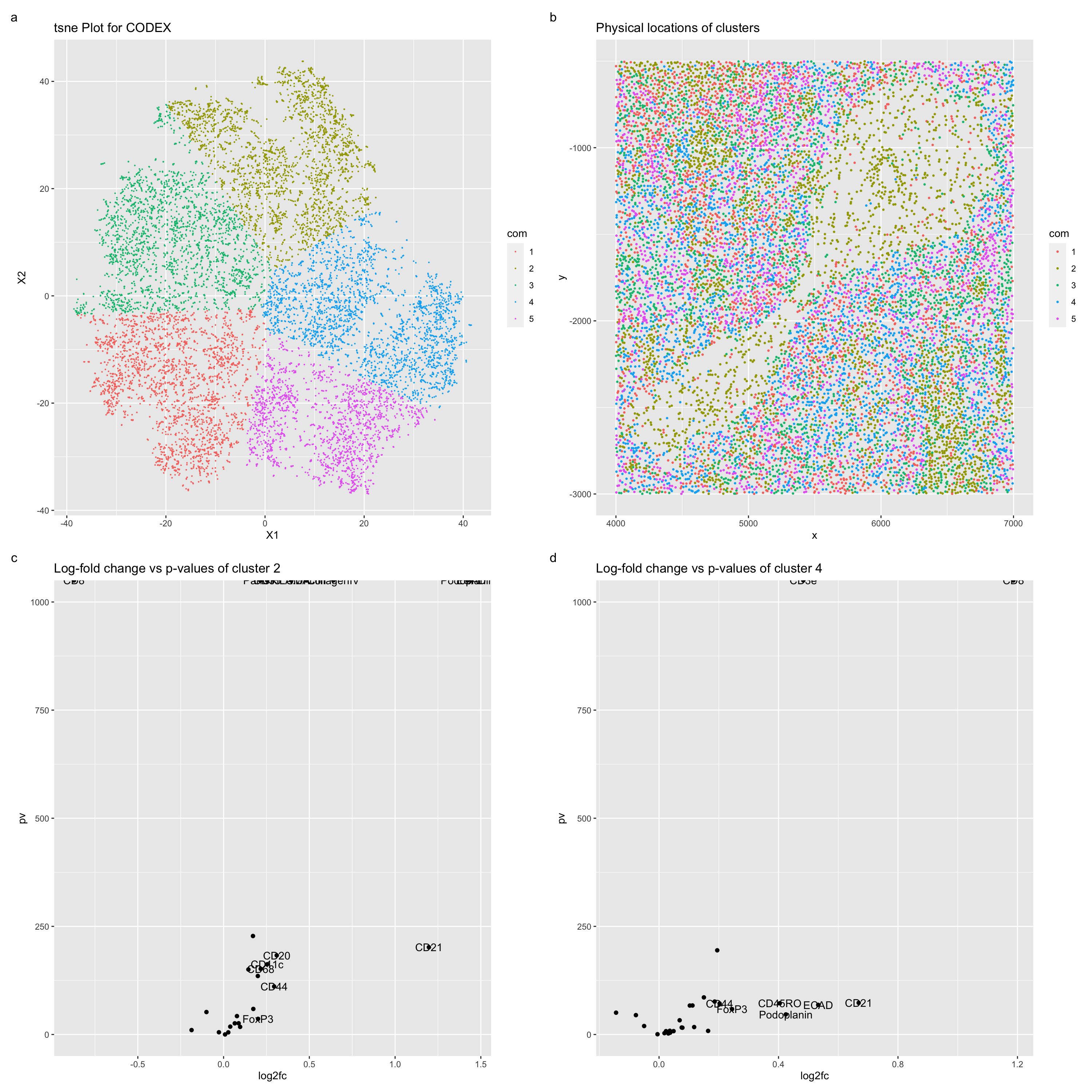
Figure Description

Figure a describes a TSNE plot for the CODEX data, with the color hues used to represent the kmeans clustering of this plot with a k = 5. Figure b describes the spatial locations of these clustered cells. Figure c describes a volcano plot for comparison of the protein expression in cells of cluster 2, and figure d describes a volcano plot for comparison of the protein expression of cells in cluster 4. Upregulated genes expressed in proteins of cluster 4 include, notably, CD8 and CD3e. These proteins are especially expressed in cytotoxic T cells (https://www.ncbi.nlm.nih.gov/books/NBK26926/#:~:text=CD4%20is%20expressed%20on%20helper,(Figure%2024%2D55)) and especially in lymphatic tissues (https://www.ncbi.nlm.nih.gov/gene/916). Lymphatic tissue is especially found in splenic regions, which encompasses white pulp (https://training.seer.cancer.gov/anatomy/lymphatic/components/spleen.html#:~:text=The%20white%20pulp%20is%20lymphatic,such%20as%20lymphocytes%20and%20macrophages). One especially upregulated cluster 2 protein is collagen IV. Collagen IV is especially common in dermal-epidermal junctions (https://www.ncbi.nlm.nih.gov/pmc/articles/PMC3289483/#:~:text=Collagen%20IV%20is%20the%20primary,found%20in%20the%20lamina%20densa.), and thus can be assumed to be more likely cells in veins/arteries (https://www.ncbi.nlm.nih.gov/books/NBK26848/).

#Code used from code-lesson-12
data <- read.csv('~/OneDrive/Documents/School/Johns Hopkins/Spring 2024/codex_spleen_subset.csv.gz', 
                 row.names=1)
head(data)
dim(data)

pos <- data[, 1:2]
area <- data[, 3]
pexp <- data[, 4:31]
head(pexp)

## plot x,y coordinates and visualize area
library(ggplot2)
df <- data.frame(pos, area)
ggplot(df) + geom_point(aes(x=x, y=y, col=area), size=0.1)

## normalize the protein expression data
hist(log10(colSums(pexp)+1))
hist(log10(rowSums(pexp)+1))
plot(log10(area+1), log10(rowSums(pexp)+1), pch=".")

#Normalization
pexp.norm <- log10(pexp/rowSums(pexp) * mean(rowSums(pexp))+1)


## kmeans clustering
tw <- sapply(1:40, function(i) {
  kmeans(pexp.norm, centers=i)$tot.withinss
})

#clustering
plot(tw, type='o')

## dimensionality reduction
pvar <- apply(pexp.norm, 2, var)
pmean <- apply(pexp.norm, 2, mean)
sort(apply(pexp.norm, 2, var))

pcs <- prcomp(pexp.norm)
head(pcs$x)

plot(pcs$sdev[1:50])
emb <- Rtsne::Rtsne(pexp.norm)$Y
#emb <- Rtsne::Rtsne(pcs$x[,1:12])$Y
head(emb)

## get clusters
tw <- sapply(1:20, function(i) {
  print(i)
  kmeans(emb, centers=i)$tot.withinss
})

tsne_clustering_elbow <- plot(tw, type='o')

com <- as.factor(kmeans(emb, centers=5)$cluster)
#tsne plot
df <- data.frame(emb, com=com)

tsne <- ggplot(df) + geom_point(aes(x = X1, y = X2, col=com), size=0.1)

#positional clusters
df <- data.frame(pos, com=com)
phys <- ggplot(df) + geom_point(aes(x = x, y = y, col=com), size=0.5)

phys

## differential expression for cluster 2
pvals <- sapply(colnames(pexp), function(p) {
  print(p)
  test <- t.test(pexp.norm[com == 2, p], pexp.norm[com != 2, p])
  test$p.value
})
fc <- sapply(colnames(pexp), function(p) {
  print(p)
  mean(pexp.norm[com == 2, p])/mean(pexp.norm[com != 2, p])
})

vals2 <- pvals

df <- data.frame(pv = -log10(pvals), log2fc = log2(fc))
#label=colnames(pexp)

head(df)

df$genes <- colnames(pexp)

# code from Caleb Hallinan
df$delabel <- ifelse(df$log2fc > .2, df$genes, NA)
df$delabel <- ifelse(df$log2fc < -.2, df$genes, df$delabel)

df$delabel

df$label 

cluster_2 <- ggplot(df) + geom_point(aes(x = log2fc, y = pv)) + 
  geom_text(aes(x = log2fc, y = pv, label = delabel)) + 
  scale_y_continuous(limits=c(0,1000))
  #+ geom_vline(xintercept = c(-1, 1), col = "gray", linetype = 'dashed') 
  #+ geom_hline(yintercept = -log10(0.05), col = "gray", linetype = 'dashed') 
cluster_2

## differential expression for cluster 4
pvals <- sapply(colnames(pexp), function(p) {
  print(p)
  test <- t.test(pexp.norm[com == 4, p], pexp.norm[com != 4, p])
  test$p.value
})

vals4 <- pvals

fc <- sapply(colnames(pexp), function(p) {
  print(p)
  mean(pexp.norm[com == 4, p])/mean(pexp.norm[com != 4, p])
})

df <- data.frame(pv = -log10(pvals), log2fc = log2(fc))
#label=colnames(pexp)

head(df)

df$genes <- colnames(pexp)

# code from Caleb Hallinan
df$delabel <- ifelse(df$log2fc > .2, df$genes, NA)
df$delabel <- ifelse(df$log2fc < -.2, df$genes, df$delabel)

df$delabel

df$label 

df

cluster_4 <- ggplot(df) + geom_point(aes(x = log2fc, y = pv)) + 
  geom_text(aes(x = log2fc, y = pv, label = delabel)) +
  scale_y_continuous(limits=c(0,1000))
#+ geom_vline(xintercept = c(-1, 1), col = "gray", linetype = 'dashed') 
#+ geom_hline(yintercept = -log10(0.05), col = "gray", linetype = 'dashed') 
cluster_4

library(patchwork)

tsne <- tsne + ggtitle("tsne Plot for CODEX")
phys <- phys + ggtitle("Physical locations of clusters")
cluster_2 <- cluster_2 + ggtitle("Log-fold change vs p-values of cluster 2")
cluster_4 <- cluster_4 + ggtitle("Log-fold change vs p-values of cluster 4")

tsne + phys + cluster_2 + cluster_4 + plot_annotation(tag_levels = 'a')