Identification of Red Pulp Tissue Structure within CODEX Dataset

Figure Description:

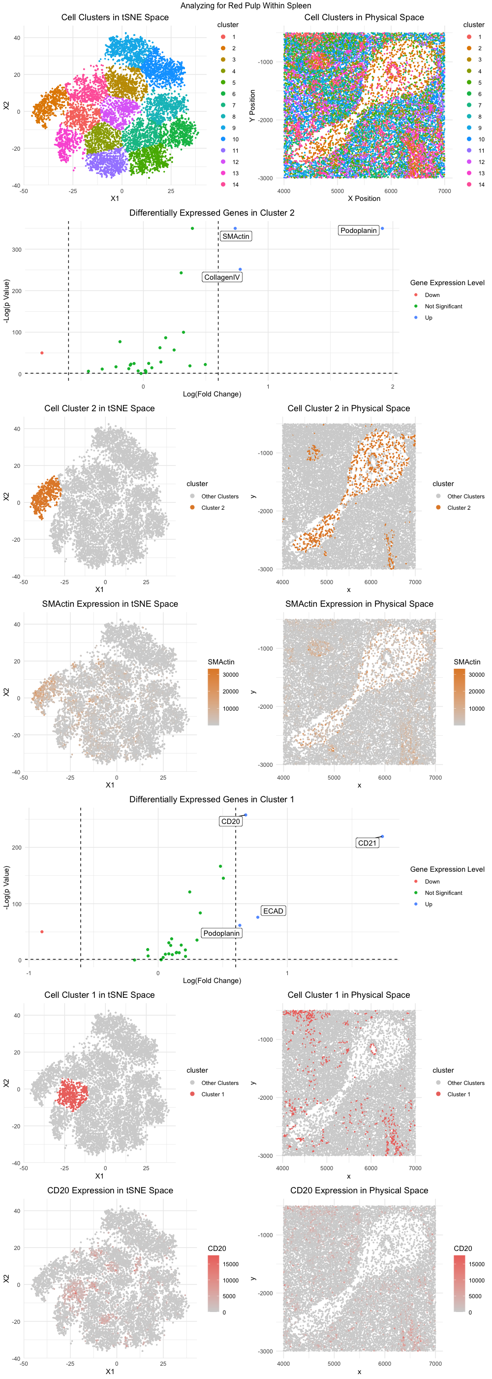
The general workflow from homework 5 was applied with some modifications, namely utilizing tSNE instead of PCA for dimensionality reduction, to analyze the CODEX dataset. I ultimately believe I have identified two clusters containing distinct cell types, with cluster 2 containing endothelial cells and cluster 1 containing lymphocytes. The locations of cluster 1 and cluster 2 in both physical and tSNE space can be examined within the visualization.

Cluster 2 had differentially upregulated CollagenIV, SMActin, and Podoplanin, as can be noted in the associated volcano plot. These proteins make me believe cluster 2 is composed of endothelial cells. Collagen IV is a major component of the basement membrane, a specialized extracellular matrix structure that provides structural support to endothelial cells and other tissue layers. In the context of endothelial cells, Collagen IV helps maintain the integrity and stability of blood vessel walls, contributing to their barrier function and regulating the passage of molecules and cells between the bloodstream and surrounding tissues [1]. Upregulation of Collagen IV expression is often indicative of endothelial cell activation or differentiation. SMActin, or smooth muscle actin, is a cytoskeletal protein typically expressed by smooth muscle cells but can also be found in certain subsets of endothelial cells, particularly those associated with blood vessels exhibiting contractile properties such as arterioles and venules [2]. Podoplanin is a transmembrane glycoprotein that plays diverse roles in various physiological and pathological processes, including lymphangiogenesis, cell migration, and tumor metastasis [3]. In the context of endothelial cells, podoplanin is primarily associated with lymphatic endothelial cells, where it contributes to the formation and maintenance of lymphatic vessels.

Cluster 1 had differentially upregulated CD20 and CD21, as can be noted in the associated volcano plot. These proteins make me believe cluster 1 is composed of lymphocytes. CD20, also known as B-lymphocyte antigen CD20, is a cell surface protein predominantly expressed by B cells, a type of lymphocyte responsible for antibody production and humoral immune responses [4]. CD20 plays a crucial role in B cell development, activation, and proliferation. It is commonly used as a marker to identify and characterize B cells in various tissues and biological samples. Similarly, CD21, also known as complement receptor type 2 (CR2), is another cell surface protein primarily expressed by B cells [5]. CD21 functions as a receptor for complement components C3d and C3dg and plays a crucial role in B cell activation, antigen presentation, and immune complex clearance.

The presence of both endothelial cells and lymphocytes strongly suggests that the CODEX dataset contains the tissue structure of red pulp within the spleen. Red pulp is a major component of the spleen responsible for blood filtration and immune surveillance. It is characterized by a network of sinusoids lined with endothelial cells, interspersed with splenic cords containing various immune cells, including lymphocytes [6]. Endothelial cells, as observed in Cluster 2, are crucial components of the sinusoidal network within the red pulp. Their presence indicates the vascular nature of the tissue and suggests that the dataset captures regions associated with blood circulation and filtration. The upregulation of markers such as Collagen IV, SMActin, and Podoplanin further supports the identification of endothelial cells, as these proteins are associated with endothelial function and vascular integrity. On the other hand, the presence of lymphocytes, as indicated by the upregulation of CD20 and CD21 in Cluster 1, is characteristic of the immune cell composition within the red pulp. Lymphocytes, particularly B cells, are abundant in the red pulp and play essential roles in immune responses, including antibody production and antigen presentation.

References:

[1] 10.1152/ajpcell.00059.2011

[2] 10.1007/s002400000165

[3] 10.1182/blood.2019001388

[4] 10.1126/scitranslmed.aaa4802

[5] 10.1093/cei/uxac103

[6] 10.1007/s00276-017-1893-0

# Load necessary packages
library(factoextra)
library(NbClust)
library(cluster)
library(ggrepel)
library(ggplot2)
library(gridExtra)
library(dplyr)
library(patchwork)
library(Rtsne)

# Load in the data
data <- read.csv("codex_spleen_subset.csv.gz", row.names = 1)
head(data)

pos <- data[,1:2]
area <- data[,3]
pexp <- data[,4:31]

# Filter the cells first for meaningful expression
cell_keep <- rownames(pexp)[rowSums(pexp) > 0]
pos <- pos[cell_keep,]
pexp <- pexp[cell_keep,]

# Normalize gene expression
total_pexp <- rowSums(pexp)
norm_pexp <- (pexp/total_pexp) * median(total_pexp)
norm_pexp <- log10(norm_pexp + 1)

# Set seed to get reproducible outputs
set.seed(8)

# Run tSNE analysis on data
emb <- Rtsne(norm_pexp, check = F)

# Determine best number of k centroids for kMeans
withinnes_values <- sapply(c(5:20), function(k) { 
  tmp = kmeans(emb$Y, centers = k)
  return(tmp$tot.withinss)
})

elbow_plot <- ggplot(data.frame(k = c(5:20), tot_withinss = withinnes_values), 
                aes(k, tot_withinss)) +
  geom_point()

elbow_plot

# Determine best number of k
opt_k <- 14

# Set seed to get reproducible outputs of kMeans
set.seed(8)

# Run kMeans clustering
kmean_cluster <- kmeans(emb$Y, centers = opt_k)
df_cluster <- data.frame(pos, cluster = as.factor(kmean_cluster$cluster), pexp, emb$Y)

# Visualize the clusters in tSNE space
tSNE_cluster <- ggplot(data = df_cluster, aes(x = X1, y = X2, col = cluster)) + 
  geom_point(size = 0.5) + 
  theme_minimal() + 
  labs(title = "Cell Clusters in tSNE Space") + 
  theme(plot.title = element_text(hjust = 0.5)) + 
  guides(color = guide_legend(override.aes = list(size = 2.5)))

tSNE_cluster

# Visualize the clusters in physical space
physical_cluster <- ggplot(data = df_cluster, aes(x = x, y = y, col = cluster)) + 
  geom_point(size = 0.5) + 
  theme_minimal() + 
  labs(title = "Cell Clusters in Physical Space", x = "X Position", y= "Y Position") + 
  theme(plot.title = element_text(hjust = 0.5)) + 
  guides(color = guide_legend(override.aes = list(size = 2.5)))

physical_cluster

#########################################################################################################

# Pick cluster 2 to analyze

# Visualize cluster 2 in tSNE
tSNE_cluster2 <- ggplot(data = df_cluster, aes(x = X1, y = X2, col = cluster == 2)) + 
  geom_point(size = 0.5) + 
  theme_minimal() + 
  labs(title = "Cell Cluster 2 in tSNE Space") + 
  theme(plot.title = element_text(hjust = 0.5)) + 
  guides(color = guide_legend(override.aes = list(size = 2.5))) + 
  scale_color_manual(name = "cluster", values = c('lightgrey', '#E28A32'), labels = c("Other Clusters", "Cluster 2"))

tSNE_cluster2

# Visualize cluster 2 in physical space
physical_cluster2 <- ggplot(data = df_cluster, aes(x = x, y = y, col = cluster == 2)) + 
  geom_point(size = 0.5) + 
  theme_minimal() + 
  labs(title = "Cell Cluster 2 in Physical Space") + 
  theme(plot.title = element_text(hjust = 0.5)) + 
  guides(color = guide_legend(override.aes = list(size = 2.5))) + 
  scale_color_manual(name = "cluster", values = c('lightgrey', '#E28A32'), labels = c("Other Clusters", "Cluster 2"))

physical_cluster2

# Volcano Plot Creation

# Identify cells that are within cluster 2 and not within cluster 2
cluster2_cells <- df_cluster[df_cluster$cluster == 2,]
not_cluster2_cells <- df_cluster[df_cluster$cluster != 2,]

# Use Wilcox test to find differentially expressed genes within cluster 2
diff_genes_2 <- sapply(colnames(pexp), function(g) {
  wilcox.test(norm_pexp[row.names(cluster2_cells), g],
              norm_pexp[row.names(not_cluster2_cells), g])$p.value
})

# Calculate statistics for volcano plot
# ratio for fold change
fc_2 <- sapply(colnames(pexp), function(g) {
  log2( mean(norm_pexp[row.names(cluster2_cells), g]) 
        / mean(norm_pexp[row.names(not_cluster2_cells), g]))
})

volcano_df_2 <- data.frame(fc_2, p = ifelse(is.infinite(-log10(diff_genes_2)), 350, -log10(diff_genes_2)))

upreg_genes_2 <- sapply(colnames(pexp), function(g) {
  wilcox.test(norm_pexp[row.names(cluster2_cells), g],
              norm_pexp[row.names(not_cluster2_cells), g],
              alternative = 'greater')$p.value
})

top_genes_2 <- names(which(upreg_genes_2 < 0.05 & fc_2 > 0.6))
top_genes_2 <- upreg_genes_2[top_genes_2]
top_genes_2 # include CollagenIV, SMActin, Podoplanin

volcano_df_2$express <- "Not Significant"
volcano_df_2$express[volcano_df_2$fc_2 > 0.6 & volcano_df_2$p > -log10(0.05)] <- "Up"
volcano_df_2$express[volcano_df_2$fc_2 < -0.6 & volcano_df_2$p > -log10(0.05)] <- "Down"

# Now plot the volcano plot
volcano_plot_2 <- ggplot(volcano_df_2) + 
  geom_point(aes(x = fc_2, y = p, col = express)) + 
  geom_hline(yintercept = -log10(0.05), linetype = "dashed") + 
  geom_vline(xintercept = c(-0.6, 0.6), linetype = "dashed") +
  geom_label_repel(data = volcano_df_2[names(top_genes_2),],
                   aes(x = fc_2, y = p, label = names(top_genes_2)), 
                   max.overlaps = 40) + 
  theme_minimal() + 
  labs(title = "Differentially Expressed Genes in Cluster 2", x = "Log(Fold Change)", y = "-Log(p Value)", col = "Gene Expression Level") + 
  theme(plot.title = element_text(hjust = 0.5))

volcano_plot_2

# Plot SMActin (most significant gene)
genetSNE_plot_2 <- ggplot(data = df_cluster) + 
  geom_point(aes(x = X1, y = X2, col = SMActin), size = 0.5) + 
  theme_minimal() + 
  scale_color_gradient(low = "lightgrey", high = "#E28A32") + 
  labs(title = "SMActin Expression in tSNE Space") + 
  theme(plot.title = element_text(hjust = 0.5))

genetSNE_plot_2

gene2d_plot_2 <- ggplot(df_cluster) + 
  geom_point(aes(x = x, y = y, col = SMActin), size = 0.5) + 
  theme_minimal() + 
  scale_color_gradient(low = "lightgrey", high = "#E28A32") + 
  labs(title = "SMActin Expression in Physical Space") + 
  theme(plot.title = element_text(hjust = 0.5))

gene2d_plot_2

#########################################################################################################

# Pick cluster 1 to analyze

# Visualize cluster 1 in tSNE
tSNE_cluster1 <- ggplot(data = df_cluster, aes(x = X1, y = X2, col = cluster == 1)) + 
  geom_point(size = 0.5) + 
  theme_minimal() + 
  labs(title = "Cell Cluster 1 in tSNE Space") + 
  theme(plot.title = element_text(hjust = 0.5)) + 
  guides(color = guide_legend(override.aes = list(size = 2.5))) + 
  scale_color_manual(name = "cluster", values = c('lightgrey', '#ED746D'), labels = c("Other Clusters", "Cluster 1"))

tSNE_cluster1

# Visualize cluster 1 in physical space
physical_cluster1 <- ggplot(data = df_cluster, aes(x = x, y = y, col = cluster == 1)) + 
  geom_point(size = 0.5) + 
  theme_minimal() + 
  labs(title = "Cell Cluster 1 in Physical Space") + 
  theme(plot.title = element_text(hjust = 0.5)) + 
  guides(color = guide_legend(override.aes = list(size = 2.5))) + 
  scale_color_manual(name = "cluster", values = c('lightgrey', '#ED746D'), labels = c("Other Clusters", "Cluster 1"))

physical_cluster1

# Volcano Plot Creation

# Identify cells that are within cluster 1 and not within cluster 1
cluster1_cells <- df_cluster[df_cluster$cluster == 1,]
not_cluster1_cells <- df_cluster[df_cluster$cluster != 1,]

# Use Wilcox test to find differentially expressed genes within cluster 1
diff_genes_1 <- sapply(colnames(pexp), function(g) {
  wilcox.test(norm_pexp[row.names(cluster1_cells), g],
              norm_pexp[row.names(not_cluster1_cells), g])$p.value
})

# Calculate statistics for volcano plot
# ratio for fold change
fc_1 <- sapply(colnames(pexp), function(g) {
  log2( mean(norm_pexp[row.names(cluster1_cells), g]) 
        / mean(norm_pexp[row.names(not_cluster1_cells), g]))
})

volcano_df_1 <- data.frame(fc_1, p = ifelse(is.infinite(-log10(diff_genes_1)), 350, -log10(diff_genes_1)))

upreg_genes_1 <- sapply(colnames(pexp), function(g) {
  wilcox.test(norm_pexp[row.names(cluster1_cells), g],
              norm_pexp[row.names(not_cluster1_cells), g],
              alternative = 'greater')$p.value
})

top_genes_1 <- names(which(upreg_genes_1 < 0.05 & fc_1 > 0.6))
top_genes_1 <- upreg_genes_1[top_genes_1]
top_genes_1 # Includes CD20, Podoplanin, CD21, ECAD

volcano_df_1$express <- "Not Significant"
volcano_df_1$express[volcano_df_1$fc_1 > 0.6 & volcano_df_1$p > -log10(0.05)] <- "Up"
volcano_df_1$express[volcano_df_1$fc_1 < -0.6 & volcano_df_1$p > -log10(0.05)] <- "Down"

# Now plot the volcano plot
volcano_plot_1 <- ggplot(volcano_df_1) + 
  geom_point(aes(x = fc_1, y = p, col = express)) + 
  geom_hline(yintercept = -log10(0.05), linetype = "dashed") + 
  geom_vline(xintercept = c(-0.6, 0.6), linetype = "dashed") +
  geom_label_repel(data = volcano_df_1[names(top_genes_1),],
                   aes(x = fc_1, y = p, label = names(top_genes_1)), 
                   max.overlaps = 40) + 
  theme_minimal() + 
  labs(title = "Differentially Expressed Genes in Cluster 1", x = "Log(Fold Change)", y = "-Log(p Value)", col = "Gene Expression Level") + 
  theme(plot.title = element_text(hjust = 0.5))

volcano_plot_1

# Plot CD20
genetSNE_plot_1 <- ggplot(data = df_cluster) + 
  geom_point(aes(x = X1, y = X2, col = CD20), size = 0.5) + 
  theme_minimal() + 
  scale_color_gradient(low = "lightgrey", high = "#ED746D") + 
  labs(title = "CD20 Expression in tSNE Space") + 
  theme(plot.title = element_text(hjust = 0.5))

genetSNE_plot_1 

gene2d_plot_1 <- ggplot(df_cluster) + 
  geom_point(aes(x = x, y = y, col = CD20), size = 0.5) + 
  theme_minimal() + 
  scale_color_gradient(low = "lightgrey", high = "#ED746D") + 
  labs(title = "CD20 Expression in Physical Space") + 
  theme(plot.title = element_text(hjust = 0.5))

gene2d_plot_1

## Combine plots together
lay <- rbind(c(1,2),
             c(3,3),
             c(4,5),
             c(6,7),
             c(8,8),
             c(9,10),
             c(11,12))

grid.arrange(tSNE_cluster, physical_cluster,
             volcano_plot_2,
             tSNE_cluster2, physical_cluster2,
             genetSNE_plot_2, gene2d_plot_2,
             volcano_plot_1,
             tSNE_cluster1, physical_cluster1,
             genetSNE_plot_1, gene2d_plot_1,
             layout_matrix = lay,
             top = "Analyzing for Red Pulp Within Spleen")

# References
# Elbow Method in R: https://www.statology.org/elbow-method-in-r/
# Volcano plot was done in conjunction / simiar research with classmate Jonathan