Using SEraster on Xenium Breast Cancer Data

Brief Description

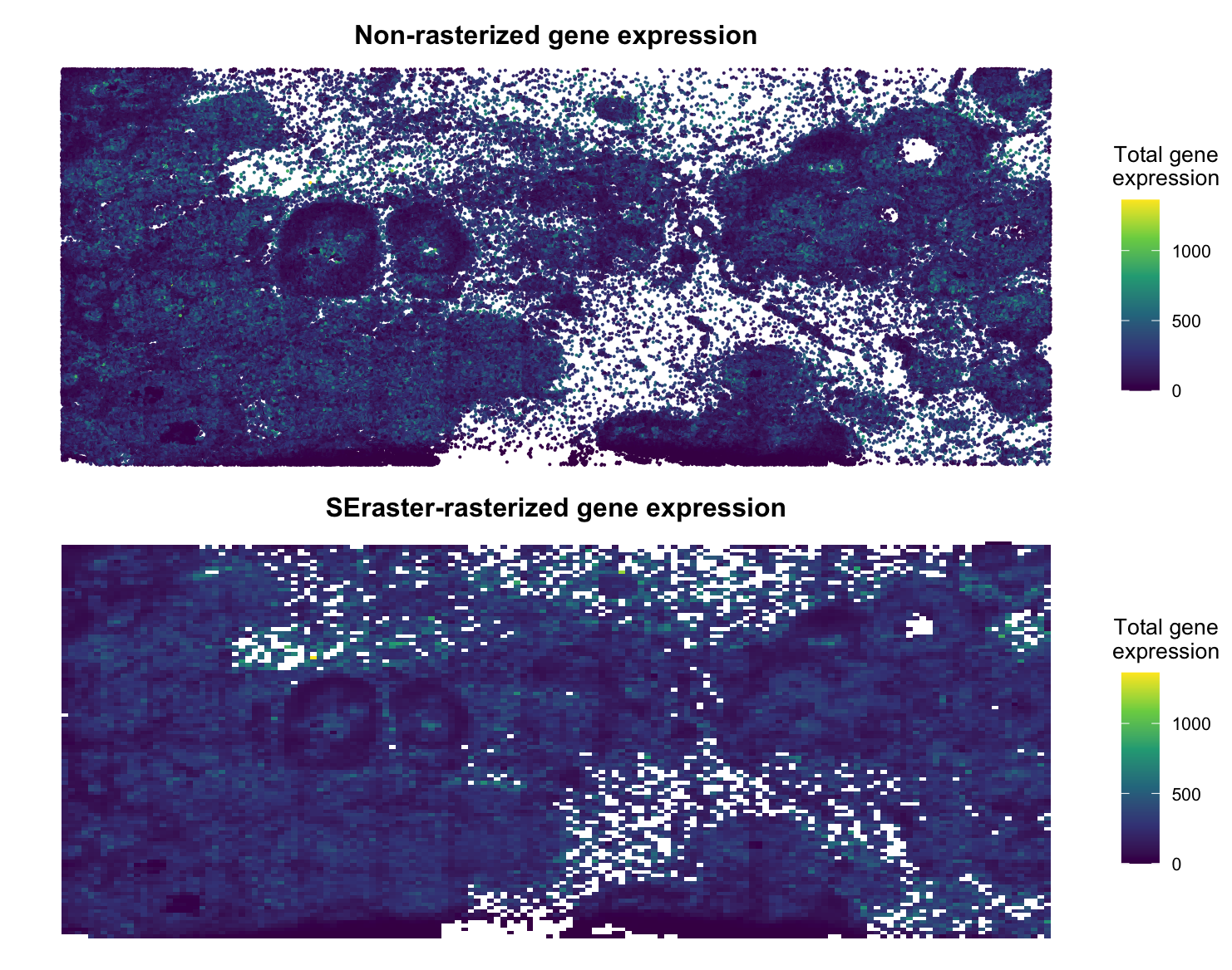
I decided to utilize SEraster on a Xenium breast cancer dataset (https://www.10xgenomics.com/products/xenium-in-situ/preview-dataset-human-breast) to rasterize gene expression. Plotted below is the non-rasterized gene expression compared to the rasterized gene expression from SEraster. I used color (hue) to express the total gene expression for both plots, where purple represents a low expression and yellow represents a high expression (viridis scale). Overall, we see very similar patterns in the data and so I would assume downstream analysis would be similar as well.

Note: This is raw counts data, so I did not normalize the data. Further, I used a resolution of 50 when applying SEraster.

Code

### Test SEraster on data ###
## 03/04/2024 ##
#  Reference: https://github.com/pachterlab/SFEData/blob/main/inst/scripts/make-data.R

# install SEraster
# require(remotes)
# remotes::install_github('JEFworks-Lab/SEraster')

# load packages
library(SpatialExperiment)
library(SEraster)
library(Seurat)
library(here)
library(SingleCellExperiment)
library(SpatialFeatureExperiment)
library(DropletUtils)
library(vroom)
library(sf)
library(scuttle)
library(scater)
library(arrow)
library(dplyr)
library(stringr)
library(patchwork)


# set seed
set.seed(02052024)


### Needed functions for reading in Xenium data ###

# Read in Xenium data and create an SFE object
readXenium <- function(dir_name){
    # Find the files
    counts_path <- paste0( dir_name, "cell_feature_matrix.h5")
    cell_info_path <- paste0( dir_name, "cells.csv.gz")
    cell_poly_path <- paste0( dir_name, "cell_boundaries.parquet")
    nuc_poly_path <- paste0( dir_name, "nucleus_boundaries.parquet")
    
    # Read in the data
    sce <- read10xCounts(counts_path)
    counts(sce) <- as(realize(counts(sce)), "dgCMatrix")
    cell_info <- vroom(cell_info_path)
    
    cell_schema <- schema(cell_id=string(),
                          vertex_x=float64(),
                          vertex_y=float64())
    
    cell_poly <- open_dataset(cell_poly_path,
                              schema=cell_schema) %>%
        collect()
    nuc_poly <- open_dataset(nuc_poly_path,
                             schema=cell_schema) %>%
        collect()
    
    names(cell_poly)[1] <- "ID"
    names(nuc_poly)[1] <- "ID"
    
    # change df to sf object for cell/nuc images
    cells_sf <- df2sf(cell_poly, c("vertex_x", "vertex_y"), geometryType = "POLYGON")
    nuc_sf <- df2sf(nuc_poly, c("vertex_x", "vertex_y"), geometryType = "POLYGON")
    
    # QC check
    all(st_is_valid(cells_sf))
    all(st_is_valid(nuc_sf))
    
    # get rid if invalid cells/nucs
    ind_invalid <- !st_is_valid(nuc_sf)
    nuc_sf[ind_invalid,] <- nngeo::st_remove_holes(st_buffer(nuc_sf[ind_invalid,], 0))
    
    # add cell info
    colData(sce) <- cbind(colData(sce), cell_info)
    print(cell_info)
    
    # make spatial objects
    spe <- toSpatialExperiment(sce, spatialCoordsNames = c("x_centroid", "y_centroid"))
    sfe <- toSpatialFeatureExperiment(spe)
    
    # add segmented cells/nuc to spatial object
    cellSeg(sfe, withDimnames = FALSE) <- cells_sf
    nucSeg(sfe, withDimnames = FALSE) <- nuc_sf
    
    
    # Add some QC Metrics
    colData(sfe)$nCounts <- colSums(counts(sfe))
    colData(sfe)$nGenes <- colSums(counts(sfe) > 0)
    
    is_blank <- str_detect(rownames(sfe), "^BLANK_")
    is_neg <- str_detect(rownames(sfe), "^NegControlProbe")
    is_neg2 <- str_detect(rownames(sfe), "^NegControlCodeword")
    is_anti <- str_detect(rownames(sfe), "^antisense")
    is_depr <- str_detect(rownames(sfe), "^DeprecatedCodeword")
    
    is_any_neg <- is_blank | is_neg | is_neg2 | is_anti | is_depr
    rowData(sfe)$is_neg <- is_any_neg
    
    n_panel <- nrow(sfe) - sum(is_any_neg)
    #print(n_panel)
    
    # normalize counts after QC
    colData(sfe)$nCounts_normed <- sfe$nCounts/n_panel
    colData(sfe)$nGenes_normed <- sfe$nGenes/n_panel
    colData(sfe)$prop_nuc <- sfe$nucleus_area / sfe$cell_area
    
    # add QC columns
    sfe <- addPerCellQCMetrics(sfe, subsets = list(blank = is_blank,
                                                   negProbe = is_neg,
                                                   negCodeword = is_neg2,
                                                   anti = is_anti,
                                                   depr = is_depr,
                                                   any_neg = is_any_neg))
    
    # add features
    rowData(sfe)$means <- rowMeans(counts(sfe))
    rowData(sfe)$vars <- rowVars(counts(sfe))
    rowData(sfe)$cv2 <- rowData(sfe)$vars/rowData(sfe)$means^2
    
    
    # Add cell ids and make gene names unique
    colnames(sfe) <- seq_len(ncol(sfe))
    rownames(sfe) <- uniquifyFeatureNames(ID=rownames(sfe),  names=rowData(sfe)$Symbol)
    
    return(sfe)
}

# convert objects
SFEtoSPE <- function(sfe){
    # First convert to an SCE
    sce <- SingleCellExperiment(assays=list(counts=counts(sfe)))
    colData(sce) <- colData(sfe)
    
    # Get the x and y centroids for this region, and add them to the coldata
    sce$x_centroid <- spatialCoords(sfe)[,1]
    sce$y_centroid <- spatialCoords(sfe)[,2]
    
    # Convert to SPE
    spe <- toSpatialExperiment(sce, spatialCoordsNames=c("x_centroid", "y_centroid"))
    
    return(spe)
}



### Read in Data ###

# read in using function
spe <- readXenium("~/Desktop/jhu/fanlab/projects/histology_to_gene_prediction/data/xenium_sample1/outs/")
# convert from spatial feature experiment to spatial experiment
sce <- SFEtoSPE(spe)



### Plot the data ###

# create df with spatial coordinates and total counts
df <- data.frame(x = spatialCoords(sce)[,1], y = spatialCoords(sce)[,2], counts = colData(sce)$total_counts)

# plot using ggplot
p <- ggplot(df, aes(x = x, y = y, color = counts)) +
    geom_point(size = 0.05) +
    theme_void() +
    labs(
        title = "Non-rasterized gene expression",
        color = "Total gene\nexpression"
    ) +
    scale_color_viridis_c() +
    theme(legend.title.align=0.5,plot.title = element_text(hjust = 0.5, face="bold", size=12),
    text = element_text(size = 10))



### Run SEraster ###

# rasterize gene expression
rastGexp <- SEraster::rasterizeGeneExpression(sce, assay_name="counts", resolution = 50)

# create a column of total counts
colData(rastGexp)$total_counts <- colSums(assay(rastGexp))

# check the dimension of the genes-by-cells matrix after rasterizing gene expression
dim(rastGexp)

# plot total rasterized gene expression
p_se <- SEraster::plotRaster(rastGexp, name = "Total rasterized gene expression", plotTitle = "SEraster-rasterized gene expression") + theme(legend.title.align=0.5,plot.title = element_text(hjust = 0.5, face="bold", size=12), text = element_text(size = 10))

# plot rasterized gene expression
# create df with spatial coordinates and total counts
df_seraster <- data.frame(x = spatialCoords(rastGexp)[,1], y = spatialCoords(rastGexp)[,2], counts = colData(rastGexp)$total_counts)

# plot using ggplot
p_se <- ggplot(df_seraster, aes(x = x, y = y, fill = counts)) +
    geom_tile() +
    theme_void() +
    labs(
        title = "SEraster-rasterized gene expression",
        fill = "Total gene\nexpression"
    ) +
    scale_fill_viridis_c() +
    theme(legend.title.align=0.5,plot.title = element_text(hjust = 0.5, face="bold", size=12),
    text = element_text(size = 10))


# plot using patchwork
p + p_se + plot_layout(nrow = 2)