gganimate: Visualizing IGKC in tSNE Space with Non-linear Dimensionality Reduction on Varying Numbers of PCs

What data types are you visualizing?

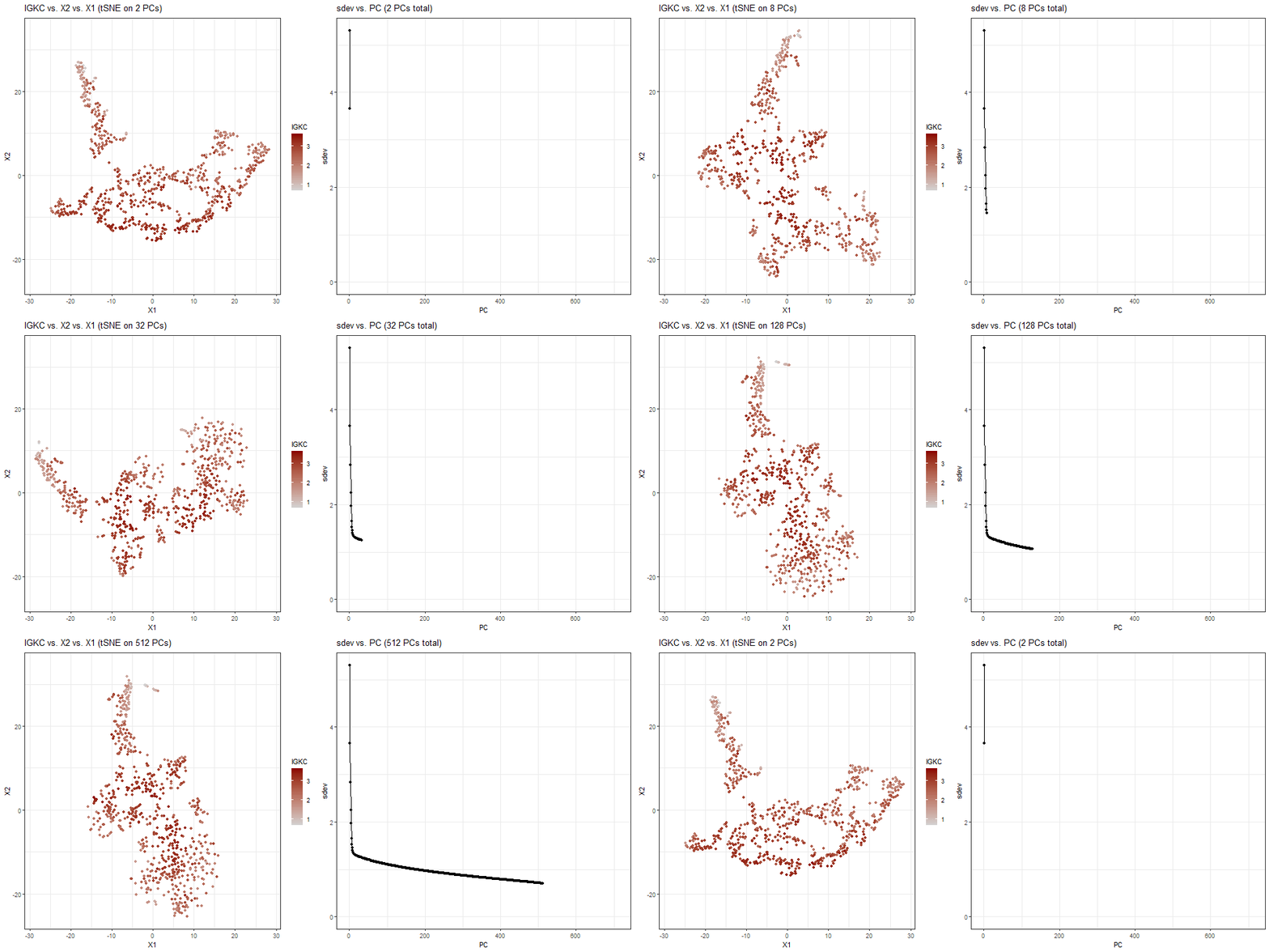
For the plots on the left side of the animation, I am visualizing the quantitative data of the X1 and X2 tSNE embedding values, and qualitative data of the IGKC expression for each spot.

For the plots on the right side of the animation, I am visualizing quantitative data of the standard deviation of the principal component, and ordinal data of the number assigned to the principal component.

What data encodings are you using to visualize these data types?

For the plots on the left side of the animation, I am using the geometric primitive of points to represent each spot on the spatial gene expression slide. To encode the X1 embedding value, I am using the visual channel of position along the x axis. To encode the X2 value, I am using the visual channel of position along the y axis. To encode the quantitative IGKC expression, I am using the visual channel of saturation going from an unsaturated light grey to a saturated red.

For the plots on the right side of the animation, I am using the geometric primitive of points to represent each principal component. To encode the quantitative standard deviation of the principal component, I am using the visual channel of position along the x axis. To encode the ordinal number assigned to the principal component, I am using the visual channel of position along the y axis.

The visual channels were chosen because according to the data type chart, position has the best resolving time, so it was used for the X1 and X2 embedding values, PC standard deviation, and PC ordinal number. Saturation was chosen to encode IGKC expression because it has a moderate resolving time for quantitative data and would not result in overlap between points in the tSNE plot, like area would.

What type of data visualization is this? What about the data are you trying to make salient through this data visualization? What Gestalt principles have you applied towards achieving this goal if any?

The plots on the left side of the animation are scatterplots. The plots on the right side of the animation are line plots.

My explanatory data visualization seeks to make more salient the effect of the number of PCs used on the output of nonlinear dimensionality reduction in tSNE space. It also makes salient the IGKC expression for each spot in tSNE space, with the saturation channel used for IGKC expression helping viewers track various groups of spots across frames of the animation. The visualization also makes salient the standard deviation for each principal component, such that the viewer can gauge how the changes in the tSNE plot from using more PCs relates to the standard deviation of those PCs.

The Gestalt principles of proximity and similarity are present because the tSNE spatial plot and standard deviation using the same number of PCs are adjacent to each other throughout the animation. The Gestalt principle of continuity is used because the frames of the animation are in increasing order for the number of PCs used for tSNE and the standard deviation plot.

Please share the code you used to reproduce this data visualization.

data <-
    read.csv("genomic-data-visualization-2024/data/eevee.csv.gz",
             row.names = 1)
data[1:10, 1:10]
pos <- data[, 2:3]
gexp <- data[, 4:ncol(data)]

# from lesson 5
topgene <- names(sort(apply(gexp, 2, var), decreasing = TRUE)[1:1000])
gexpfilter <- gexp[, topgene]


# code taken from Dr. Fan's code-lesson-5.R
# gexpnorm <- log10(gexpfilter/rowSums(gexpfilter) * mean(rowSums(gexpfilter))+1)
gexpnorm <- log10(gexp/rowSums(gexp) * mean(rowSums(gexp))+1)

? prcomp
pcs <- prcomp(gexpnorm)
plot(pcs$sdev, type = 'o')

library(ggplot2)
ggplot(data.frame(pos, gexpnorm)) + 
    scale_colour_gradient(low = 'lightgrey', high = 'darkred') +
    geom_point(aes(x= aligned_x, y=aligned_y, color = IGKC)) + 
    theme_minimal()

? Rtsne
library(Rtsne)

nsteps = ceiling(log2(length(pcs$sdev)))
sdev_plts <- list()
tsne_plts <- list()
df_anim <- data.frame()
df_sdev <- data.frame()
for (i in 1:nsteps) {
    npcs = 2^i
    
    s <- ""
    if (npcs > length(pcs$sdev)) {
        npcs = length(pcs$sdev)
        s <- "all "
    }
    
    print(paste(i, npcs))
    
    sdev_df = data.frame(sdev = pcs$sdev[1:npcs])
    
    sdev_df$PC = as.numeric(rownames(sdev_df))
    
    sdev_plts[[i]] <- ggplot(sdev_df, aes(x = PC, y = sdev, grouping = 1)) + 
        geom_point() + geom_line() + 
        labs(
            title = sprintf(
                'sdev vs. PC (%d PCs total)',
                npcs
            )
        ) +
        theme_bw()

    set.seed(42)
    emb <- Rtsne(pcs$x[,1:npcs])$Y
    
    df <- data.frame(emb, gexpnorm)
    df_anim <- rbind(df_anim, cbind(df, npcs = npcs))
    df_sdev <- rbind(df_sdev, cbind(sdev_df, npcs = npcs))
    
    tsne_plts[[i]] <-
        ggplot(df) + geom_point(aes(x = X1, y = X2, color = IGKC)) +
        scale_colour_gradient(low = 'lightgrey', high = 'darkred') +
        labs(
            title = sprintf(
                'IGKC vs. X2 vs. X1 (tSNE on %s%d PCs)',
                s,
                npcs
            )
        ) +
        theme_bw()
}
    
sdev_plts[[1]]
tsne_plts[[10]]

library(gganimate)
main_plt <- ggplot(df_anim) + geom_point(aes(x = X1, y = X2, color = IGKC)) +
    scale_colour_gradient(low = 'lightgrey', high = 'darkred') +
    labs(
        title = 'IGKC vs. X2 vs. X1 (tSNE on {closest_state} PCs)'
    ) +
    theme_bw()
main_anim <- main_plt + 
    transition_states(npcs,
            state_length = 2,
            transition_length = 1) +
    ease_aes('sine-in-out')

sdev_plt <- ggplot(df_sdev, aes(x = PC, y = sdev, grouping = 1)) + 
    geom_point() + geom_line() + 
    labs(
        title = 
            'sdev vs. PC ({closest_state} PCs total)'
        
    ) +
    theme_bw()
sdev_anim <- sdev_plt + 
    transition_states(npcs,
                      state_length = 2,
                      transition_length = 1) +
    ease_aes('sine-in-out')

main_gif <- animate(main_anim, renderer = magick_renderer())
sdev_gif <- animate(sdev_anim, renderer = magick_renderer())

i=1
new_gif <- image_append(c(main_gif[i], sdev_gif[i]))
for(i in 2:100){
    combined <- image_append(c(main_gif[i], sdev_gif[i]))
    new_gif <- c(new_gif, combined)
}

new_gif

image_write(new_gif, "aying2.gif")