Cell Cluster Identification and Validation in Breast Tumor Tissue (revised)

Plot Description
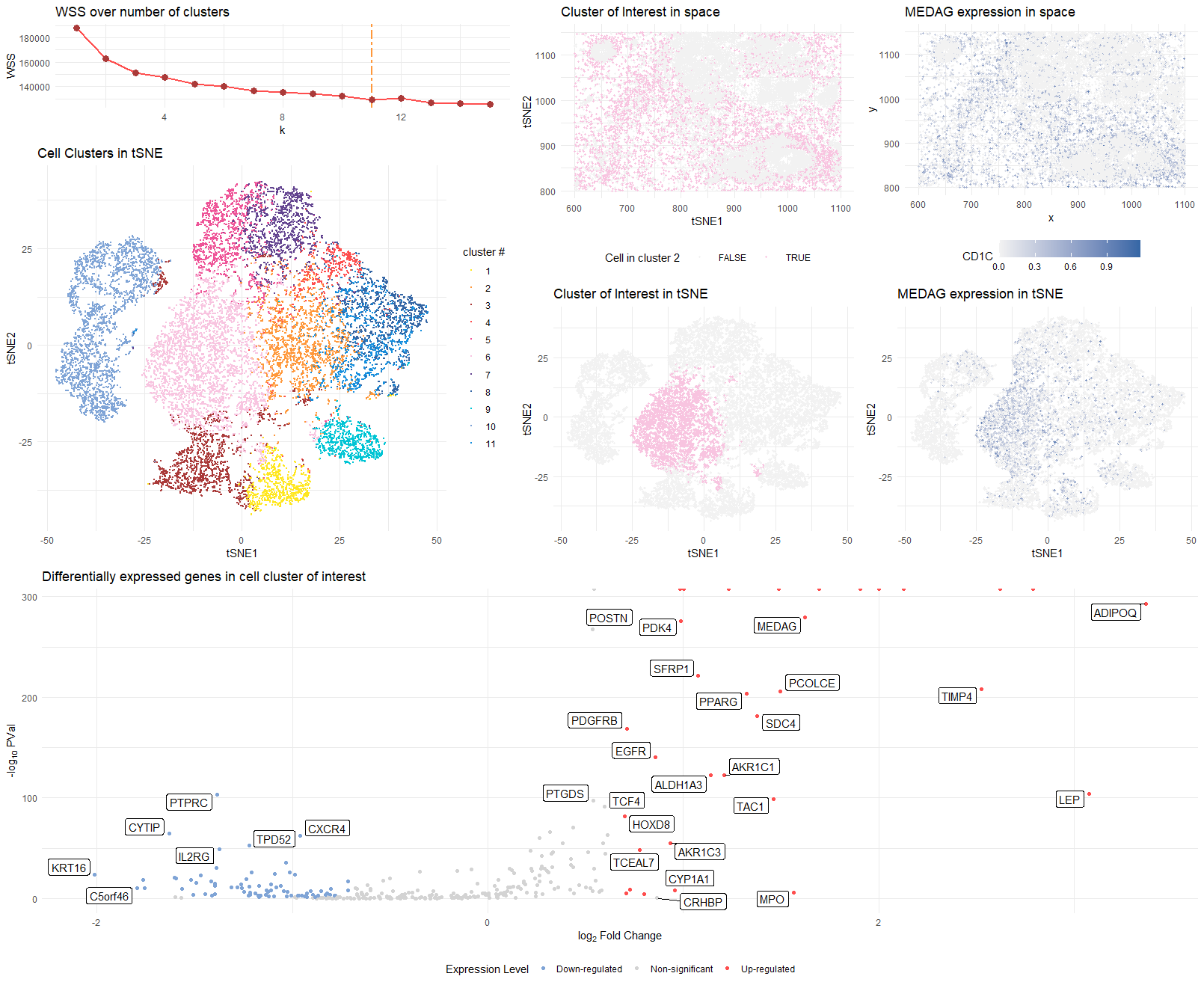
This visualization presents differential gene expression to validate cell type identification by k-means on 2D tSNE space.
-
The spatial-transcriptomics data on breast tumor tissue is preprocessed by removing cells with total gene counts below 10, normalized by total gene counts, and log-scaled.
-
The 10 cell clusters (see WSS curve for choice of k) are encoded by different colors in tSNE space to show the perfomance of k-means clustering. Number of clusters are revised to 11 instead of 10.
-
Cluster 6 is selected as cluster of interest and identified in both tSNE and physical space with the same color used in the 10-cluster plot.
-
The most differentially expressed genes are computed in the selected cluster through two-sided Wilcox test, and demonstrated on the volcano plot.
-
The signature MEDAG () gene’s distribution is plotted in both tSNE and physical space
Cluster of Interest
The selected cluster of interest is highly possible to be stromal cells that contains a subtype of adipocytes.
- Up-regulated MEDAG MEDAG, or Mesenteric estrogen-dependent adipogenesis gene, was first reported as a novel adipogenic gene1. It has been found to be highly expressed in breast cancer samples (making it a more reliable identifier.
MEDAG was newly identified as an adipogenic gene capable of promoting differentiation of preadipocytes into adipocytes. In mature adipocytes, upregulation of MEDAG could increase lipid content and promote glucose up-taking [1].
-
Up-regulated ADIPOQ ADIPOQ, or Adiponectin, is also associated with breast cancer. A study found that several cancer-associated adipocyte subtypes, namely DPP4+ adipocytes in visceral adipose and ADIPOQ+ adipocytes in subcutaneous adipose, are identified. High levels of these sub-types are associated with unfavorable outcomes in four typical adipose-associated cancers [2].
-
Evidence for more than diopocytes:
- contains more cells than MEDAG-expressing cells
- expression of TIMP4 (more common in smooth muscle cells)
- physical distribution surrounds more organized structures/clusters - mechanical support
References
[1] Yang J, Yu P. Identification of MEDAG as a Hub Candidate Gene in the Onset and Progression of Type 2 Diabetes Mellitus by Comprehensive Bioinformatics Analysis. Biomed Res Int. 2021 Feb 25;2021:3947350. doi: 10.1155/2021/3947350. PMID: 33728329; PMCID: PMC7938259.
[2] Liu, SQ., Chen, DY., Li, B. et al. Single-cell analysis of white adipose tissue reveals the tumor-promoting adipocyte subtypes. J Transl Med 21, 470 (2023). https://doi.org/10.1186/s12967-023-04256-7
[3] https://www.10xgenomics.com/products/xenium-in-situ/human-breast-dataset-explorer
Source Code
## load dataset
data <- read.csv('C:/Users/ivych/OneDrive - Johns Hopkins/Classes/Data Visualization/pikachu.csv.gz', row.names = 1)

# install.packages("Rtsne")
## import libraries
library(ggplot2)
library(gridExtra)
library(Rtsne)

## set theme
plot_theme <- theme_bw() +
  theme(text = element_text(size = 10), legend.key.size = unit(0.5, 'cm'))
#ref: https://www.color-hex.com/color-palette/1022322
xiao_plt <- c( "#ffe720",
               "#FF983B",
               "#AA3A39",
               "#FE4E4E",
               "#EE5397",
               "#f8c4e0",
               "#634490",
               "#3466A5",
               "#00C4D4",
               "#7fa4d6",
               "#158edd")

## data selection
pos <- data[,4:5]
gexp <- data[,6:ncol(data)]
good.cells <-rownames(gexp)[rowSums(gexp) > 10]
pos <- pos[good.cells,]
gexp <- gexp[good.cells,]

## normalization
gexp_norm <- gexp*median(rowSums(gexp))/rowSums(gexp)
gexp_log <- log10(gexp_norm+1)
mat <- unique(gexp_log)

#scree plot for pcs
x <- 1:15
pcs <- prcomp(mat)
par(mfrow=c(1,1))
data_scree <- data.frame(x = x, std = pcs$sdev[1:15])
ggplot(data_scree, aes(x, std)) +
  geom_line(color = xiao_plt[4], size = 1) +
  geom_point(color = xiao_plt[3], size = 3) +
  labs(title = "Scree plot", x = "Number of PCs", y = "STD") +
  theme_minimal()
#pcs = 8

#pcs and tsne
pcs_result <- pcs$x[,1:8]
tsne_result <- Rtsne::Rtsne(pcs_result)

## elbow method for clustering
wss <- numeric(15)
for (i in 1:15) {
  wss[i] <- sum(kmeans(mat, centers = i)$withinss)
}
data_elbow <- data.frame(x = x, wss = wss)
p_elbow <- ggplot(data_elbow, aes(x, wss)) +
  geom_segment(col = xiao_plt[2], size=1, linetype = 'twodash',
               aes(x = 11, y = Inf, xend = 11, yend = -Inf)) +
  geom_line(color = xiao_plt[4], size = 1) +
  geom_point(color = xiao_plt[3], size = 3) +
  labs(title = "WSS over number of clusters", x = "k", y = "WSS") +
  theme_minimal()
p_elbow

## K-means
#k = 11 seems to give the optimal result (modified)
com = kmeans(mat, center  = 11)
df <- data.frame(pos, tsne_result$Y, celltype=as.factor(com$cluster))
head(df)
p_k <- ggplot(df) +
  geom_point(size = 0.4,aes(x = X1, y = X2, col=celltype)) +
  labs(title = 'Cell Clusters in tSNE',
       x = 'tSNE1', y = 'tSNE2', col = "cluster #") +
  theme_minimal() + # theme(legend.position = "none") +
  scale_colour_manual(values = xiao_plt)
p_k
# pick cluster of interest - same one with last submission
coi <- 6

#cluster of interest in the tsne space
p_c1 <- ggplot(df) +
  geom_point(size = 0.7,aes(x = X1, y = X2, col=(celltype==coi))) +
  labs(title = 'Cluster of Interest in tSNE',
       x = 'tSNE1', y = 'tSNE2',col="in cluster 2") +
  theme_minimal() + theme(legend.position = "none") +
  scale_colour_manual(values = c("grey95",xiao_plt[coi]))
p_c1

#cluster of interest in the physical space
p_c2 <- ggplot(df) +
  geom_point(size = 0.7, aes(x = aligned_x, y = aligned_y, col=(celltype==coi))) +
  labs(title = 'Cluster of Interest in space',
       x = 'tSNE1', y = 'tSNE2',col="Cell in cluster 2") +
  theme_minimal() + theme(legend.position = "bottom", legend.key.size = unit(1, "cm")) +
  scale_colour_manual(values = c("grey95",xiao_plt[coi]))
p_c2

## Double-sided wilcox test to identify differential expression
cluster.oi<- names(which(com$cluster == coi))
cluster.ot <- names(which(com$cluster != coi))

#differential genes
genes <- colnames(mat)
pvs <- sapply(genes, function(g) {
  oi <- mat[cluster.oi, g]
  ot <- mat[cluster.ot, g]
  wilcox.test(oi, ot, alternative="two.sided")$p.val})

names(which(pvs < 1e-100))
head(sort(pvs), n=15)

#fold change
log2fc <- sapply(genes, function(g) {
  oi <- mat[cluster.oi, g]
  ot <- mat[cluster.ot, g]
  log2(mean(oi)/mean(ot))})

#volcano plot
df_volcano <- data.frame(pvs, log2fc)
exp_sig <- apply(df_volcano, 1, function(g) {
  if (g[2] >= log(2) & g[1] <= 0.05) {out = "Up-regulated"}
  else if (g[2] <= -log(2) & g[1] <= 0.05) {out = "Down-regulated"}
  else {out = "Non-significant"}
  out})
data_deg <- cbind(df_volcano, exp_sig)

#install.packages("ggrepel")

p_volc <- ggplot(data_deg, aes(y=-log10(pvs), x=log2fc)) +
  scale_color_manual(values = c(xiao_plt[10], "lightgray", xiao_plt[4])) +
  geom_point(aes(col = exp_sig)) +
  ggrepel::geom_label_repel(label=rownames(data_deg)) +
  xlab(expression("log"[2]*" Fold Change")) +
  ylab(expression("-log"[10]*" PVal")) +
  theme_minimal()+
  theme(legend.position = 'bottom') +
  labs(title = 'Differentially expressed genes in cell cluster of interest',
       col = "Expression Level")

p_volc

# Visualize CD1C
# https://bmccancer.biomedcentral.com/articles/10.1186/s12885-023-10558-2#:~:text=CD1C%20is%20an%20important%20part%20of%20the%20TME,and%20a%20new%20treatment%20target%20for%20breast%20cancer.

df_cd1c <- cbind(df,CD1C = mat$MEDAG)

p_cd1c1 <-ggplot(df_cd1c) +
  geom_point(size = 0.8,aes(x = aligned_x, y = aligned_y, col = CD1C)) +
  theme_minimal() + theme(legend.position="bottom", legend.key.width = unit(1, "cm")) +
  labs(title = 'MEDAG expression in space',
       x = 'x', y = 'y') +
  scale_color_gradient(low = 'grey95', high=xiao_plt[8])
p_cd1c1

p_cd1c2 <- ggplot(df_cd1c) +
  geom_point(size = 0.8,aes(x = X1, y = X2, col = CD1C)) +
  theme_minimal()+ theme(legend.position="none", legend.key.size = unit(0.2, "cm")) +
  labs(title = 'MEDAG expression in tSNE',
       x = 'tSNE1', y = 'tSNE2') +
  scale_color_gradient(low = 'grey95', high=xiao_plt[8])
p_cd1c2


#plot panel arrangement
layout <- rbind(c(1,1,1,3,3,4,4),
                c(2,2,2,3,3,4,4),
                c(2,2,2,5,5,6,6),
                c(2,2,2,5,5,6,6),
                c(7,7,7,7,7,7,7),
                c(7,7,7,7,7,7,7),
                c(7,7,7,7,7,7,7))
grid.arrange(p_elbow,p_k,
             p_c2,p_cd1c1,
             p_c1,p_cd1c2,
             p_volc,
             layout_matrix = layout)