Identifying Type of Tissue in the Spleen
You will need to visualize and interpret at least two cell-types. Create a data visualization and write a description to convince me that your interpretation is correct.
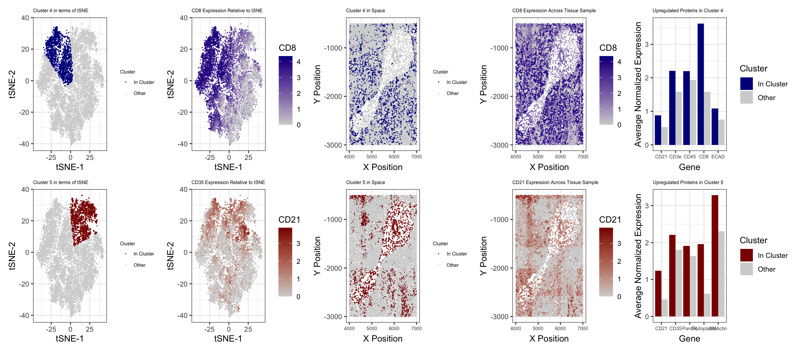
To determine the type of tissue, I first log transformed and normalized protein expression, before performing PCA and tSNE. I then checked total withiness for different k values for clustering based on tSNE, and I found that 5 was the optimal number of clusters. After conducting k means clustering with 5 centers, I used Wilcoxon tests on clusters 4 and 5 to determine proteins with upregulated expression. I then looked into proteins with the smallest p values for each of these clusters to determine their cell types. I plotted each cluster in both physical space as well as relative to tSNE. I also plotted an upregulated gene for each cluster (CD8 for cluster 4, CD21 for 5) on X-Y and tSNE coordinates. I also plotted average expression in and out of the cluster of interest for 5 upregulated proteins with the lowest p values for each cluster of interest. For cluster 4, I found CD8, CD3e, CD45, CD21, and ECAD to be upregulated. From my research, I found that CD8 is a marker for T cells (1). I also found CD3e to be a subunit within T cell receptors (2), further suggesting that this cluster included T cells. CD45 is expressed in nearly all types of white blood cells (3), and CD21 is a marker for B cells and dendritic cells (4). I also found that ECAD is generally expressed in macrophages. Combining all of this, I believe that this cluster consists of T cells, along with some macrophages as well as B cells or dendritic cells. For cluster 5, I found SMActin, Podoplanin, PanCK, CD21, CD35, and HLA.DR to be upregulated. Both CD21 and CD35 are dendritic cell markers (6), and CD35 is also known to be expressed on B cells (7). Podoplanin is also known to be expressed in dendritic cells (8). HLA is expressed in antigen presenting cells, including B cells, macrophages, and dendritic cells (9). Actin is also highly expressed in dendritic cells (10). Collectively, this suggests that this cluster is mostly dendritic cells, with potentially also some B cells and macrophages. When looking into the different types of tissue in the spleen, I found that white pulp contains lymphocytes including T cells and B cells, as well as macrophages, all arranged around arteries (11). Additionally, dendritic cells are abundant in the white pulp as well (12). Given that the protein expression data suggests that all of these cell types are present in the tissue sample, I believe that this tissue is white pulp. The conformation of cells around an opening in the middle would also align with the fact that white pulp is around arteries.
Sources:
- https://www.ncbi.nlm.nih.gov/pmc/articles/PMC2118473/
- https://www.ncbi.nlm.nih.gov/gene/916
- https://pubmed.ncbi.nlm.nih.gov/9429890
- https://ashpublications.org/blood/article/115/3/519/27130/Differential-expression-of-CD21-identifies
- https://pubmed.ncbi.nlm.nih.gov/26226941
- https://www.ncbi.nlm.nih.gov/pmc/articles/PMC4399542/
- https://www.ncbi.nlm.nih.gov/pmc/articles/PMC3633082
- https://www.ncbi.nlm.nih.gov/pmc/articles/PMC3439854/
- https://www.ncbi.nlm.nih.gov/books/NBK459467
- https://www.frontiersin.org/articles/10.3389/fcell.2021.679500/full
- https://www.histology.leeds.ac.uk/
- https://pubmed.ncbi.nlm.nih.gov/17944899/
library(ggplot2)
library(patchwork)
library(Rtsne)
library(dplyr)
library(reshape2)

data <- read.csv('codex_spleen_subset.csv.gz', row.names = 1)
head(data)
pos <- data[, 1:2]
area <- data[, 3]
pexp <- data[, 4:31]

## checking proteins with the greatest variance in expression
sort(apply(pexp, 2, var), decreasing=TRUE)

## plot x,y coords and visualize area
df <- data.frame(pos, area)
ggplot(df) + geom_point(aes(x=x, y=y, col = area), size = 0.1)

## normalize protein expression data

pexpnorm <- log10(pexp/rowSums(pexp) * mean(rowSums(pexp)) + 1)


## dimensionality reduction
pvar <- apply(pexpnorm, 2, var)
pmean <- apply(pexpnorm, 2, mean)
sort(apply(pexpnorm, 2, var))
pcs <- prcomp(pexpnorm)
head(pcs$x)
plot(pcs$sdev[1:20])

#tSNE
emb <- Rtsne::Rtsne(pcs$x[,1:18])$Y
head(emb)
df <- data.frame(emb, protein2 = pexpnorm$Podoplanin)
ggplot(df) + geom_point(aes(x=X1, y=X2, col = protein2), size = 0.1)

df <- data.frame(pcs$x, protein = pexpnorm$Podoplanin)
ggplot(df) + geom_point(aes(x=PC1, y=PC2, col = protein), size = 0.1)
## determining optimal cluster number
tw2 <- sapply(1:20, function(i) {
  kmeans(emb, centers=i)$tot.withinss
})
plot(tw2, type ='l')
## k means clustering with 5 centers
com <- as.factor(kmeans(emb, centers=5)$cluster)

clusters <- data.frame(pexpnorm, pos, emb, com)
## categorizing genes as in or out of cluster 4 and 5
infour <- vector('integer', 11512)
infive <- vector('integer', 11512)
for(i in 1:nrow(clusters)) {
  if(clusters$com[i] == 4) {
    infour[i] <- 1
  }
  else {
    infour[i] <- 0
  }
}

for(i in 1:nrow(clusters)) {
  if(clusters$com[i] == 5) {
    infive[i] <- 1
  }
  else {
    infive[i] <- 0
  }
}
clusters <- data.frame(clusters, infour, infive)

## cluster 4 on tSNE
p1 <- ggplot(clusters) +
  geom_point(aes(x = X1, y = X2, col = as.factor(infour)), size=0.01) +
  theme_bw() +
  scale_colour_manual(name = "Cluster", labels = c("Other", "In Cluster"), values = c("lightgrey", "darkblue")) + xlab('tSNE-1') +
  ylab('tSNE-2') + labs(title = 'Cluster 4 in terms of tSNE') +
  theme(plot.title = element_text(size = 6)) +
  guides(colour = guide_legend(reverse=TRUE)) +
  theme(legend.key.size = unit(0.5, 'cm')) +
  theme(legend.title = element_text(size=6)) +
  theme(legend.text = element_text(size=6))
p1
## cluster 4 in visual space
p2 <- ggplot(clusters) +
  geom_point(aes(x = x, y = y, col = as.factor(infour)), size = 0.02) +
  theme_bw() +
  scale_colour_manual(name = "Cluster", labels = c("Other", "In Cluster"), values = c("lightgrey", "darkblue")) +
  xlab('X Position') +
  ylab('Y Position') + labs(title = 'Cluster 4 in Space') +
  theme(plot.title = element_text(size = 6)) +
  guides(colour = guide_legend(reverse=TRUE)) +
  theme(legend.key.size = unit(0.5, 'cm')) +
  theme(legend.title = element_text(size=6)) +
  theme(legend.text = element_text(size=6)) +
  theme(axis.text.x=element_text(size=6))
p2

## cluster 5 on tSNE
p3 <- ggplot(clusters) +
  geom_point(aes(x = X1, y = X2, col = as.factor(infive)), size=0.01) +
  theme_bw() +
  scale_colour_manual(name = "Cluster", labels = c("Other", "In Cluster"), values = c("lightgrey", "darkred")) + xlab('tSNE-1') +
  ylab('tSNE-2') + labs(title = 'Cluster 5 in terms of tSNE') +
  theme(plot.title = element_text(size = 6)) +
  guides(colour = guide_legend(reverse=TRUE)) +
  theme(legend.key.size = unit(0.5, 'cm')) +
  theme(legend.title = element_text(size=6)) +
  theme(legend.text = element_text(size=6))
p3
## cluster 5 in visual space
p4 <- ggplot(clusters) +
  geom_point(aes(x = x, y = y, col = as.factor(infive)), size = 0.02) +
  theme_bw() +
  scale_colour_manual(name = "Cluster", labels = c("Other", "In Cluster"), values = c("lightgrey", "darkred")) +
  xlab('X Position') +
  ylab('Y Position') + labs(title = 'Cluster 5 in Space') +
  theme(plot.title = element_text(size = 6)) +
  guides(colour = guide_legend(reverse=TRUE)) +
  theme(legend.key.size = unit(0.5, 'cm')) +
  theme(legend.title = element_text(size=6)) +
  theme(legend.text = element_text(size=6)) +
  theme(axis.text.x=element_text(size=6))
p4

## differential expression cluster 5
p <- 'CD8'
results <- sapply(colnames(pexp), function(p) {
  print(p)
  test <- wilcox.test(pexpnorm[com == 5, p], pexpnorm[com != 5, p])
  test$p.value
})
sort(results, decreasing=FALSE)

## differential expression cluster 4
results2 <- sapply(colnames(pexp), function(p) {
  print(p)
  test <- wilcox.test(pexpnorm[com == 4, p], pexpnorm[com != 4, p])
  test$p.value
})
sort(results2, decreasing=FALSE)

## gene of interest in cluster 4
p5 <- ggplot(clusters) +
  geom_point(aes(x= X1, y = X2, col = CD8), size = 0.01 ) +
  scale_colour_gradientn(colours = c("lightgrey", "darkblue"))+
  labs(title = "CD8 Expression Relative to tSNE") + xlab('tSNE-1') +
  ylab('tSNE-2') +
  theme_bw() +
  theme(plot.title = element_text(size = 6))

p6 <- ggplot(clusters) +
  geom_point(aes(x = x, y = y, col = CD8), size = 0.01) +
  scale_colour_gradientn(colours = c("lightgrey", "darkblue"))+
  labs(title = "CD8 Expression Across Tissue Sample") + xlab('X Position') +
  ylab('Y Position') +
  theme_bw() +
  theme(plot.title = element_text(size = 6)) +
  theme(axis.text.x=element_text(size=6))
p6

## gene of interest in cluster 5
p7 <- ggplot(clusters) +
  geom_point(aes(x= X1, y = X2, col = CD21), size = 0.01 ) +
  scale_colour_gradientn(colours = c("lightgrey", "darkred"))+
  labs(title = "CD35 Expression Relative to tSNE") + xlab('tSNE-1') +
  ylab('tSNE-2') +
  theme_bw() +
  theme(plot.title = element_text(size = 6))

p8 <- ggplot(clusters) +
  geom_point(aes(x = x, y = y, col = CD21), size = 0.1) +
  scale_colour_gradientn(colours = c("lightgrey", "darkred"))+
  labs(title = "CD21 Expression Across Tissue Sample") + xlab('X Position') +
  ylab('Y Position') +
  theme_bw() +
  theme(plot.title = element_text(size = 6)) +
  theme(axis.text.x=element_text(size=6))
p7
p8
## pulling out proteins with smallest p vals, cluster 4
prots4 <- as.data.frame(sort(results2, decreasing=FALSE)[1:5])
topprots4 <- data.frame(matrix(ncol = 3, nrow = 5))
colnames(topprots4) <- c('prot','clusterexp','otherexp')
## finding average normalized expression of proteins in vs out of cluster 4
for(i in 1:nrow(topprots4)) {
  topprots4$prot[i] <- rownames(prots4)[i]
  topprots4$clusterexp[i] <- mean(pexpnorm[com == 4, rownames(prots4)[i]])
  topprots4$otherexp[i] <- mean(pexpnorm[com != 4, rownames(prots4)[i]])
}

df2 <- melt(topprots4, id.vars='prot')
p9 <- ggplot(df2, aes(x=prot, y=value, fill=variable)) +
  geom_bar(stat='identity', position='dodge') +
  scale_fill_manual(name = 'Cluster', labels = c("In Cluster", "Other"), values = c("darkblue", "lightgrey")) +
  labs(title = "Upregulated Proteins in Cluster 4") + xlab('Gene') +
  ylab('Average Normalized Expression') +
  theme_bw() +
  theme(plot.title = element_text(size = 6)) +
  theme(axis.text.x=element_text(size=6))
p9

## pulling out proteins with smallest p vals, cluster 5
prots5 <- as.data.frame(sort(results, decreasing=FALSE)[1:5])
topprots5 <- data.frame(matrix(ncol = 3, nrow = 5))
colnames(topprots5) <- c('prot','clusterexp','otherexp')
## finding average normalized expression of proteins in vs out of cluster 4
for(i in 1:nrow(topprots5)) {
  topprots5$prot[i] <- rownames(prots5)[i]
  topprots5$clusterexp[i] <- mean(pexpnorm[com == 5, rownames(prots5)[i]])
  topprots5$otherexp[i] <- mean(pexpnorm[com != 5, rownames(prots5)[i]])
}

df3 <- melt(topprots5, id.vars='prot')
p10 <- ggplot(df3, aes(x=prot, y=value, fill=variable)) +
  geom_bar(stat='identity', position='dodge') +
  scale_fill_manual(name = 'Cluster', labels = c("In Cluster", "Other"), values = c("darkred", "lightgrey")) +
  labs(title = "Upregulated Proteins in Cluster 5") + xlab('Gene') +
  ylab('Average Normalized Expression') +
  theme_bw() +
  theme(plot.title = element_text(size = 6)) +
  theme(axis.text.x=element_text(size=6))
p10

top <- p1 + p5 + p2 + p6 + p9 + plot_layout(ncol = 5)
bottom <- p3 + p7 + p4 + p8 + p10 + plot_layout(ncol=5)
top/bottom