Identification of Blood Vessel Cell Cluster in Spleen Tissue

Description of Visualization

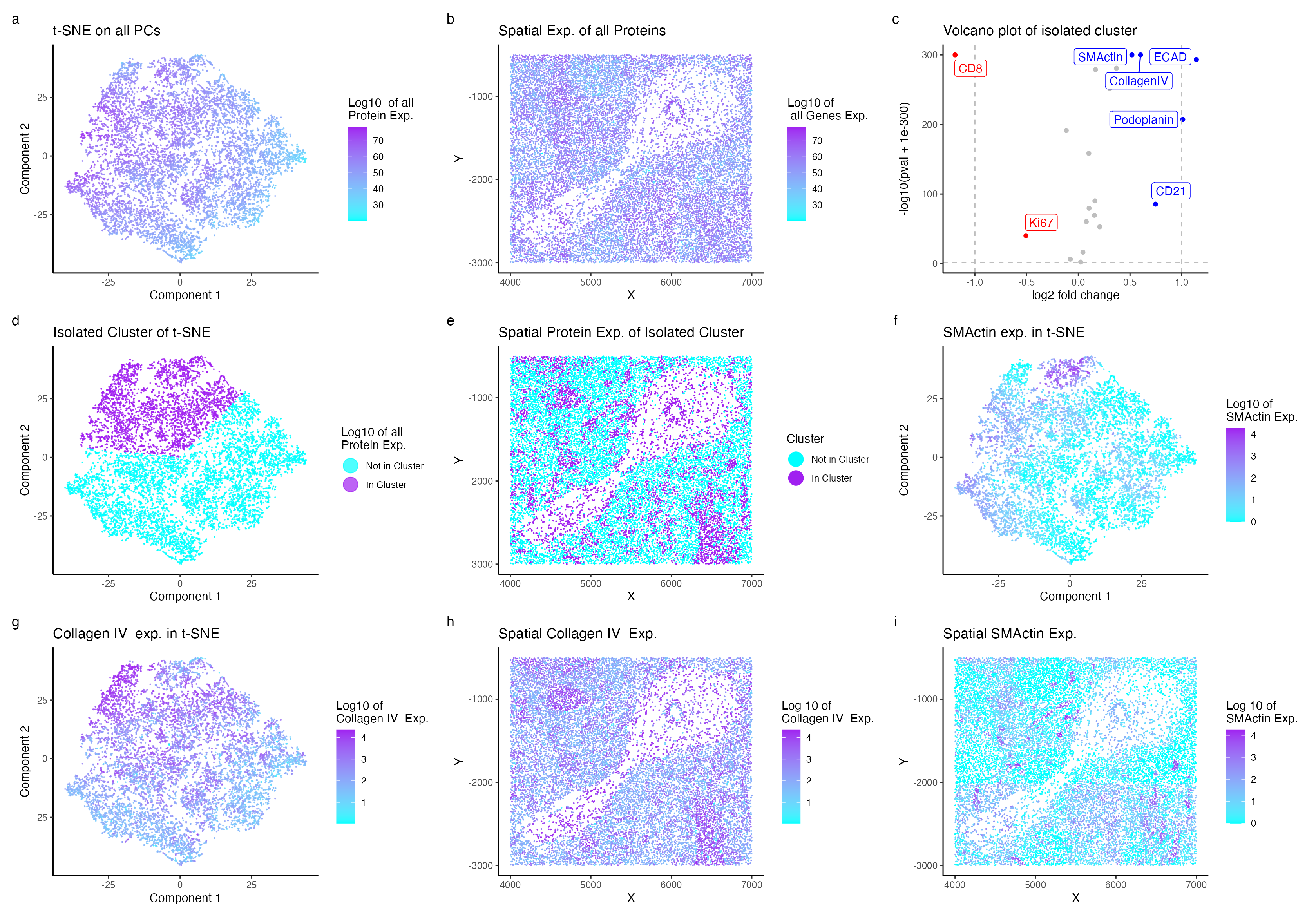
I am analyzing spleen tissue from the CODEX dataset and have identified a region composed of artery/vein cell types. Specifically, this cluster of cells expresses SMActin and Collagen IV. My visualization displays the nonlinear dimensional reduction of the principal components of the normalized protein expression. Protein expression was normalized to account for the likelihood of larger cells expressing more proteins. A clustering size of 3 folds was determined to be optimal based on both an elbow curve and visual analysis. Upregulation of ECAD, Collagen IV, SMActin, Podoplanin, and CD21 was observed in the volcano plot. The protein expression is not significantly correlated with the isolated cluster (as shown in plots d and e), likely due to the presence and function of these proteins in different cell types. However, it was determined that the combined presence of Collagen IV (as depicted in plots f and i) and SMActin (in plots f and i), along with the overall higher expression of these proteins within the cluster, is indicative of vasculature cells.

Cell Type Interpretation:

Collagen IV and Smooth Muscle Actin (SMActin) are structural regulatory proteins essential for blood vessel function. Collagen IV, a basement membrane protein, is crucial for blood vessel stability (Gross et al.), while SMActin is upregulated in blood vessels due to its ability to induce constriction (Hutter-Schmid et al.). Although both SMActin and Collagen IV are present in various cell types, their combined upregulation in vascular cells suggests blood vessel functionality within the cluster.

Gross et al.: https://www.ncbi.nlm.nih.gov/pmc/articles/PMC8487879/ Hutter-Schmid et al.:https://www.ncbi.nlm.nih.gov/pmc/articles/PMC6020076/#:~:text=Alpha%2Dsmooth%20muscle%20actin%20(%CE%B1SMA)%20is%20a%20cytoskeletal%20protein,%CE%B1SMA%20%5B13%2C14%5D.

library(Rtsne)
library(ggplot2)
library(patchwork)
library(viridis)
library(dplyr)
library(ggrepel)
set.seed(0)

data <- read.csv("/Users/knm/github/genomic-data-visualization-2024/data/codex_spleen_subset.csv.gz", row.names = 1)

gexp <- data[, 4:ncol(data)]

topgene <- names(sort(apply(gexp, 2, var), decreasing=TRUE)) 
gexp <- gexp[,topgene]

pos <- data[, 1:2]

gexpnorm <- log10(gexp/rowSums(gexp) * mean(rowSums(gexp))+1)
dim(gexp)

pcs <- prcomp(gexpnorm)
plot(pcs$sdev)
#emb <- Rtsne(pcs$x)$Y 
#emb <- Rtsne(gexpnorm)$Y 
emb <- Rtsne(pcs$x[,1:10])$Y 

calculate_wss <- function(data, k_max) {
  wss <- numeric(k_max)
  
  for (k in 1:k_max) {
    kmeans_result <- kmeans(data, centers = k, nstart = 10)
    wss[k] <- kmeans_result$tot.withinss
  }
  
  return(wss)
}
k_max <- 10
wss <- calculate_wss(emb, k_max)
elbow_point <- which(diff(diff(wss)) == min(diff(diff(wss))))
plot(1:k_max, wss, type = "b", pch = 19, frame = FALSE, 
     xlab = "Number of clusters", ylab = "Total within-cluster sum of squares")

com <- as.factor(kmeans(emb, centers=3)$cluster)
#com <- as.factor(kmeans(gexpnorm, centers=6)$cluster)
cluster_analysis <- 3

df <- data.frame(emb_1 = emb[,1], emb_2 = emb[,2],
                 com = com)

p1 <- ggplot(df) +
  geom_point(aes(x = emb_1, y = emb_2, color = com == cluster_analysis), alpha = 0.7, size = 0.1) +
  scale_color_manual(values = c("TRUE" = "purple", "FALSE" = "cyan"),
                     labels = c("Not in Cluster", "In Cluster")) +
  guides(color = guide_legend(override.aes = list(size = 6))) +
  theme_classic() +
  labs(title = "Isolated Cluster of t-SNE", color = "Log10 of all \nGenes Exp.", 
       x = "Component 1", y = "Component 2")
p1

p2 <- ggplot(df) +
  geom_point(aes(x = emb_1, y = emb_2, color = rowSums(gexpnorm)), alpha = 0.7, size = 0.1) +
  scale_color_gradient(low = "cyan", high = "purple") +
  theme_classic() +
  labs(title = "t-SNE on all PCs", color = "Log10  of all \nGenes Exp.", 
       x = "Component 1", y = "Component 2")
p2

pv <- sapply(colnames(gexpnorm), function(i) {
  wilcox.test(gexpnorm[com == cluster_analysis, i], gexpnorm[com != cluster_analysis, i], alternative = "two.sided")$p.val
})
logfc <- sapply(colnames(gexpnorm), function(i) {
  log2(mean(gexpnorm[com == cluster_analysis, i])/mean(gexpnorm[com != cluster_analysis, i]))
})

plot_df <- data.frame(logfc = logfc, pv = -log10(pv))

p3 <- ggplot(plot_df, aes(x = logfc, y = pv)) +
  geom_point() +
  theme_classic() +
  labs(title = "logFC vs PV",
       x = "Log Fold Change",
       y = "-log10(p-value)")
p3


df_spatial <- data.frame(x = pos[,1], y = pos[,2], cluster = com)
p4 <- ggplot(df_spatial) + 
  geom_point(aes(x = x, y = y, color = com == cluster_analysis), size = 0.1) +
  scale_color_manual(values = c("TRUE" = "purple", "FALSE" = "cyan"),
                     labels = c("Not in Cluster", "In Cluster")) +
  guides(color = guide_legend(override.aes = list(size = 6))) +
  theme_classic() +
  labs(title = "Spatial Exp. of Isolated Cluster", color = "Cluster", 
       x = "X", y= "Y")
p4

product <- -log10(pv) * logfc
top_genes <- names(sort(product, decreasing = TRUE))
print(top_genes)
gene_analysis <- top_genes[1]
p5 <- ggplot(df) +
  geom_point(aes(x = emb_1, y = emb_2, color = gexpnorm[,gene_analysis]), alpha = 0.7, size = 0.1) +
  scale_color_gradient(low = "cyan", high = "purple") +
  theme_classic() +
  labs(title = "CollagenIV  exp. in t-SNE", color = "Log10 of \nCollagenIV  Exp.", 
       x = "Component 1", y = "Component 2")
p5

df_spatial_2 <- data.frame(x = pos[,1], y = pos[,2], gene = gexpnorm[, gene_analysis])
p6 <- ggplot(df_spatial_2) + 
  geom_point(aes(x = x, y = y, color = gene), size = 0.1) +
  scale_color_gradient(low = "cyan", high = "purple") +
  theme_classic() +
  labs(title = "Spatial CollagenIV  Exp.", color = "Log 10 of \nCollagenIV  Exp.", 
       x = "X", y= "Y")
p6

df_spatial_3 <- data.frame(x =pos[,1], y = pos[,2], gene = rowSums(gexpnorm))
p7 <- ggplot(df_spatial_3) + 
  geom_point(aes(x = x, y = y, color = gene), size = 0.1) +
  scale_color_gradient(low = "cyan", high = "purple") +
  theme_classic() +
  labs(title = "Spatial Exp. of all Genes", color = "Log10 of \n all Genes Exp.", 
       x = "X", y= "Y")
p7


# Volcano plot 
# Ref: https://dplyr.tidyverse.org/reference/case_when.html
plot.df =  data.frame(pv = -log10(pv + 1e-300), 
                      logfc = logfc, 
                      name = colnames(gexp)) %>% 
  mutate(gene.reg = case_when( pv >1.30103 &  logfc < -0.5 ~ "Downregulated", 
                               pv >1.30103 &  logfc > 0.5 ~ "Upregulated",
                               .default  = "No_difference"))


gene.cols = c("red", "blue", "grey")
names(gene.cols) = c("Downregulated", "Upregulated", "No_difference")

#Ref: https://ggplot2.tidyverse.org/reference/geom_abline.html
#Ref: https://www.datanovia.com/en/blog/how-to-remove-legend-from-a-ggplot/

p3 <- ggplot(data =plot.df , aes(x = logfc, y = pv, col = gene.reg)) +
  geom_point()+
  geom_vline(xintercept = 1, linetype='dashed', col = 'grey') +
  geom_vline(xintercept = -1, linetype='dashed', col = 'grey') +
  geom_hline(yintercept = 1.30103, linetype='dashed', col = 'grey')+
  geom_label_repel(data=subset(plot.df, pv> 20) %>% filter(logfc <= -0.5 | logfc >=0.5 ) ,
                   aes(logfc,pv,label=name)) +
  
  theme_classic() +
  theme(legend.position = "None")+
  scale_color_manual(values = gene.cols) +
  xlab( "log2 fold change")+
  ylab("-log10(pval + 1e-300)") +
  ggtitle("Volcano plot of isolated cluster")
p3


gene_analysis2 <- top_genes[10]
p8 <- ggplot(df) +
  geom_point(aes(x = emb_1, y = emb_2, color = gexpnorm[,gene_analysis2]), alpha = 0.7, size = 0.1) +
  scale_color_gradient(low = "cyan", high = "purple") +
  theme_classic() +
  labs(title = "SMActin exp. in t-SNE", color = "Log10 of \nSMActin Exp.", 
       x = "Component 1", y = "Component 2")
p8

df_spatial_2 <- data.frame(x = pos[,1], y = pos[,2], gene = gexpnorm[, gene_analysis2], alpha = 0.7)
p9 <- ggplot(df_spatial_2) + 
  geom_point(aes(x = x, y = y, color = gene), size = 0.1) +
  scale_color_gradient(low = "cyan", high = "purple") +
  theme_classic() +
  labs(title = "Spatial SMActin Exp.", color = "Log 10 of \nSMActin Exp.", 
       x = "X", y= "Y")
p9

combined_plot <- p2 + p7 + p3 + p1 + p4 + p8 + p5 + p6 + p9 + plot_annotation(tag_levels = 'a') + 
  plot_layout(ncol = 3) #p3
combined_plot
ggsave("/Users/knm/Library/CloudStorage/OneDrive-JohnsHopkins/Johns Hopkins [2021-2025]/Junior [2023-2024]/Genomics Data Visualization/Homework/hw6_kmukund1.png", combined_plot, width = 24*.7, height = 16.70*.7, units = "in", dpi = 200)

## Volcano plot code adapted from Archana Balan's "Cell type exploration using differential gene expression analyses"