Identifying Proteins and Functional Regions in the Spleen

My hypothesis is that this data represents a section of spleen tissue which includes an artery and surrounding white pulp. My hypothesis is based off of the cell types I identified within my tissue.
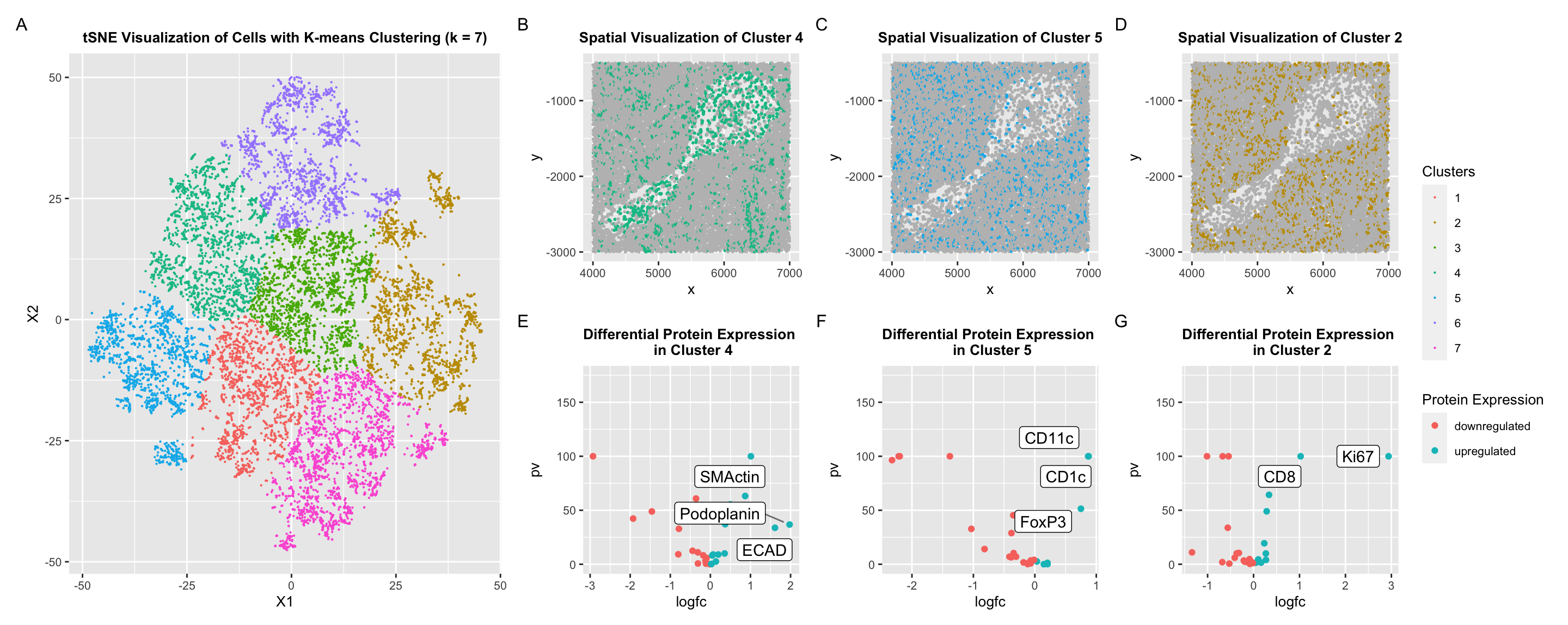
To identify cell types, I explored differential protein expression on cell clusters that I segmented using k-means clustering. First, I normalized the protein expression within each protein because different proteins may have different strengths of detection depending on antibody specificity and other factors. Then, I found that the optimal within-ness was obtained when k=7. With these clusters, I decided to analyze three different clusters.
Cluster 4 was spatially located in the cavity-like structure. In Cluster 4, SMActin, ECAD, and Podoplanin were upregulated. Smooth muscle actin is commonly found in smooth muscle cells, such as those lining the walls of blood vessels like artieries. Furthermore, E-Cadherin is a protein involved in cell adhesion, especially for epithelial cells. I was originally confused about this, but I hypothesize that VE-Cadherin (1), a vascular endothelial cadherin may instead have been detected by E-Cadherin antibodies. If this is the case, it further supports my hypothesis that this structure is an artery. Finally, podoplanin is found commonly in lymphatic endothelial cells (2). LECs are found in the white pulp. In my spatial visualization of cluster 4, some of the cells in the denser tissue surrounding the cavity were clustered with the cells in the cavity due to the k-means clustering strategy. When I visualized expression of the podoplanin protein, I found that this protein was also in the surrounding cells. While visualizing these proteins individually, I found that the expression of SMActin was not isolated to the cavity-like structure which I had originally hypothesized but rather distributed across all cells in cluster 4. Upon further research, I realized that actin beta is commonly found in white pulp (3), so it is possible that other actin proteins were also detected. Individual protein expression is not included in my final submitted visualization.
Cluster 5 showed upregulation of CD11c, CD1c, and Foxp3 proteins. CD11c is a protein that is commonly found in dendritic cells (4), which are important to inducing and controlling the adaptive immune response of T-cells. This is an important function of the white pulp, which is involved mainly with initiation of immune responses against blood-borne antigens and pathogens (5). CD1c has a similar function (6). Finally, Foxp3 is a member of the forkhead transcription factor family. It is mainly expressed in a subset of CD4+ T-cells that play a suppressive role in the immune system (7).
Cluster 2 showed upregulation of Ki67. The white pulp is primarily involved in immune responses and contains lymphoid follicles rich in B and T lymphocytes. During immune responses, both B and T lymphocytes undergo proliferation. Therefore, Ki67 expression can be observed in proliferating lymphocytes within the white pulp (8,9).
In conclusion, I believe that this is a section of spleen tissue which contains white pulp and potentially a muscular blood vessel like an artery. The presence of many cell types that facilitate T-Cell and B-cell function make me more confident in my hypothesis about the presence of white pulp. Anatomically, this structure surrounds blood vessels, and while the spatial location of proteins that may relate to blood vessels causes me to reconsider this hypothesis, the cavity makes me believe that there is a structure with a lumen. More experimentation must be done to support these conclusions, and different clustering techniques can be used in the future to have clearer segmentation of different cell types.
Citations:
- https://www.ncbi.nlm.nih.gov/pmc/articles/PMC10433914/#:~:text=Vascular endothelial (VE)-cadherin,contact between ECs is essential
- https://www.proteinatlas.org/ENSG00000162493-PDPN/single+cell+type
- https://www.proteinatlas.org/ENSG00000075624-ACTB/tissue/spleen
- https://www.sciencedirect.com/topics/immunology-and-microbiology/cd11c
- https://www.ncbi.nlm.nih.gov/pmc/articles/PMC4118229/#:~:text=The spleen contains multiple subsets,presentation to naïve T cells
- https://www.genecards.org/cgi-bin/carddisp.pl?gene=CD1C
- https://pubmed.ncbi.nlm.nih.gov/20429413/#:~:text=FOXP3 is a member of,role in the immune system
- https://www.sciencedirect.com/science/article/pii/S0006497120498416
- https://www.cell.com/cell-reports/pdf/S2211-1247(20)31365-6.pdf
##HW6
#Andrea Cheng (acheng41)

data = read.csv('~/Desktop/GDV class/data/codex_spleen_subset.csv.gz', row.names = 1)

head(data)
dim(data)

pos = data[,1:2]
area = data[,3]
pexp = data[,4:ncol(data)]

#design choices
my_color = scale_color_viridis_c(option= "C")
my_theme = theme(
  plot.title = element_text(hjust = 0.5, face="bold", size=10),
  text = element_text(size = 10)
)

#import libraries
library(ggplot2)
library(ggrepel)
library(patchwork)


#normalizing for each protein (antibodies allow comparison between cells but not
# between different proteins)
pexp_norm = log10(pexp/colSums(pexp) * mean(colSums(pexp))+1)

#plot xy coordinates
df = data.frame(pos, area)
ggplot(df) + geom_point(aes(x = x, y = y, col=area), size = 0.1)


#dimensionality reduction
#look at variance
sort(apply(pexp_norm, 2, var))
pvar= apply(pexp_norm, 2, var)
pmean = apply(pexp_norm, 2, mean)
plot(pmean, pvar)

pcs = prcomp(pexp_norm)
plot(pcs$sdev)


##nonlinear dimensionality reduction
emb = Rtsne::Rtsne(pexp_norm)$Y
# emb = Rtsne::Rtsne(pcs$x[,1:12])$Y
df = data.frame(emb)
ggplot(df) + geom_point(aes(x = X1, y = X2), size = 0.5)


#Clustering
tw = sapply(1:10, function(i) {
  kmeans(emb, centers= i)$tot.withinss
})
plot(tw, type = 'l')

coms = kmeans(emb, centers = 7)

df_spacial = data.frame(emb, pos, com = as.factor(coms$cluster))
ggplot(df_spacial) + geom_point(aes(x = x, y = y, col = com), size = 0.5)


df_emb = data.frame(emb, protein = pexp_norm$PanCK, com = as.factor(coms$cluster))
tsne_cluster = ggplot(df_emb) + geom_point(aes(x = X1, y = X2, col = com), size =0.1) +
  labs(
    title = "tSNE Visualization of Cells with K-means Clustering (k = 7)",
    col = "Clusters"
  ) + my_theme
df_protein = data.frame(pcs$x, com =as.factor(coms$cluster) )
ggplot(df_protein) + geom_point(aes(x= PC1, y = PC2, col = com), size = 0.1)


## volcano plot of cluster 4
com_categories = as.factor(coms$cluster)
pv4 = sapply(colnames(pexp_norm), function(i){
  print(i)
  wilcox.test(pexp_norm[com_categories==4, i], pexp_norm[com_categories!=4, i])$p.val
})

logfc4 = sapply(colnames(pexp_norm), function(i){
  print(i)
  log2(mean(pexp_norm[com_categories==4, i])/mean(pexp_norm[com_categories!=4, i]))
})


#create a volcano plot
df_volcano = data.frame(pv=-(log10(pv4+1e-100)),logfc =logfc4)
#add proteins as a column
df_volcano$proteins <- rownames(df_volcano)
rownames(df_volcano) <- NULL
head(df_volcano)
c4_volcano = ggplot(df_volcano) + geom_point(aes(x = logfc, y = pv,
                                    col = ifelse(logfc > 0,'upregulated', 'downregulated'))) +
  geom_label_repel(aes(x = logfc, y = pv, label=ifelse( logfc>1, as.character(proteins),NA)),
                   box.padding   = 0.35, point.padding = 0.5, segment.color = 'grey50',
                   max.overlaps = getOption("ggrepel.max.overlaps", default = 60)
  )+ ylim(-.05, 175) + labs(
    col = "Protein Expression",
    title = "Differential Protein Expression \n in Cluster 4"
  ) + my_theme


#Volcano Plot for Cluster #5
pv5 = sapply(colnames(pexp_norm), function(i){
  print(i)
  wilcox.test(pexp_norm[com_categories==5, i], pexp_norm[com_categories!=5, i])$p.val
})

logfc5 = sapply(colnames(pexp_norm), function(i){
  print(i)
  log2(mean(pexp_norm[com_categories==5, i])/mean(pexp_norm[com_categories!=5, i]))
})


#create a volcano plot
df_volcano_5 = data.frame(pv=-(log10(pv5+1e-100)),logfc =logfc5)
#add proteins as a column
df_volcano_5$proteins <- rownames(df_volcano_5)
rownames(df_volcano_5) <- NULL
head(df_volcano_5)
c5_volcano = ggplot(df_volcano_5) + geom_point(aes(x = logfc, y = pv,
                                    col = ifelse(logfc > 0,'upregulated', 'downregulated'))) +
  geom_label_repel(aes(x = logfc, y = pv, label=ifelse( logfc > 0.5, as.character(proteins),NA)),
                   box.padding   = 0.35, point.padding = 0.5, segment.color = 'grey50',
                   max.overlaps = getOption("ggrepel.max.overlaps", default = 60)
  )+ ylim(-.05, 175) + labs(
    col = "Protein Expression",
    title = "Differential Protein Expression \n in Cluster 5"
  ) + my_theme


#volcano plot for cluster #2
pv2 = sapply(colnames(pexp_norm), function(i){
  print(i)
  wilcox.test(pexp_norm[com_categories==2, i], pexp_norm[com_categories!=2, i])$p.val
})

logfc2 = sapply(colnames(pexp_norm), function(i){
  print(i)
  log2(mean(pexp_norm[com_categories==2, i])/mean(pexp_norm[com_categories!=2, i]))
})


#create a volcano plot
df_volcano_2 = data.frame(pv=-(log10(pv2+1e-100)),logfc = logfc2)
head(df_volcano_2)
#add proteins as a column
df_volcano_2$proteins <- rownames(df_volcano_2)
rownames(df_volcano_2) <- NULL
head(df_volcano_2)
c2_volcano = ggplot(df_volcano_2) + geom_point(aes(x = logfc, y = pv,
                                                   col = ifelse(logfc > 0,'upregulated', 'downregulated'))) +
  geom_label_repel(aes(x = logfc, y = pv, label=ifelse(  logfc > 1, as.character(proteins),NA)),
                   box.padding   = 0.35, point.padding = 0.5, segment.color = 'grey50',
                   max.overlaps = getOption("ggrepel.max.overlaps", default = 60)
  )+ ylim(-.05, 175) + labs(
    col = "Protein Expression",
    title = "Differential Protein Expression \n in Cluster 2"
  ) + my_theme


#spacial visualization
df_tissue = data.frame(pos,kmeans = com_categories, protein = pexp_norm$SMActin)

ggplot(df_tissue) + geom_point(aes(x = x, y = y,col = log10(protein +1)), size = 0.4)

c2_tissue = ggplot(df_tissue) + geom_point(aes(x = x, y = y,
                                   col = ifelse(kmeans == 2, 'Cluster 2', 'all other cells')), size = 0.4)+
  labs(
    col = "Cluster",
    title = "Spatial Visualization of Cluster 2"
  ) + scale_color_manual(values = c("gray", "#C49A00"))+ my_theme


c4_tissue = ggplot(df_tissue) + geom_point(aes(x = x, y = y,
                                               col = ifelse(kmeans == 4, 'Cluster 4', 'all other cells')), size = 0.4)+
  labs(
    col = "Cluster",
    title = "Spatial Visualization of Cluster 4"
  ) + scale_color_manual(values = c("gray", "#00C094"))+ my_theme

c5_tissue = ggplot(df_tissue) + geom_point(aes(x = x, y = y,
                                               col = ifelse(kmeans == 5, 'Cluster 5', 'all other cells')), size = 0.4)+
  labs(
    col = "Cluster",
    title = "Spatial Visualization of Cluster 5"
  ) + scale_color_manual(values = c("gray", "#00B6EB"))+ my_theme


tsne_cluster + (c4_tissue + theme(legend.position = "none")) + (c5_tissue + theme(legend.position = "none")) + (c2_tissue + theme(legend.position = "none")) + c4_volcano + c5_volcano + c2_volcano+
  plot_annotation(tag_levels = 'A') +
  plot_layout(guides = "collect",
              design = "
              11234
              11567
              ")