What is in a Spleen? Identifying the Tissue Structure of the CODEX dataset

Your goal is to figure out what tissue structure is represented in the CODEX data. Options include: (1) Artery/Vein, (2) White pulp, (3) Red pulp, (4) Capsule/Trabecula. You will need to visualize and interpret at least two cell-types. Create a data visualization and write a description to convince me that your interpretation is correct. Your description should reference papers and content that allowed you to interpret your cell clusters as a particular cell-types
Overview of Analysis
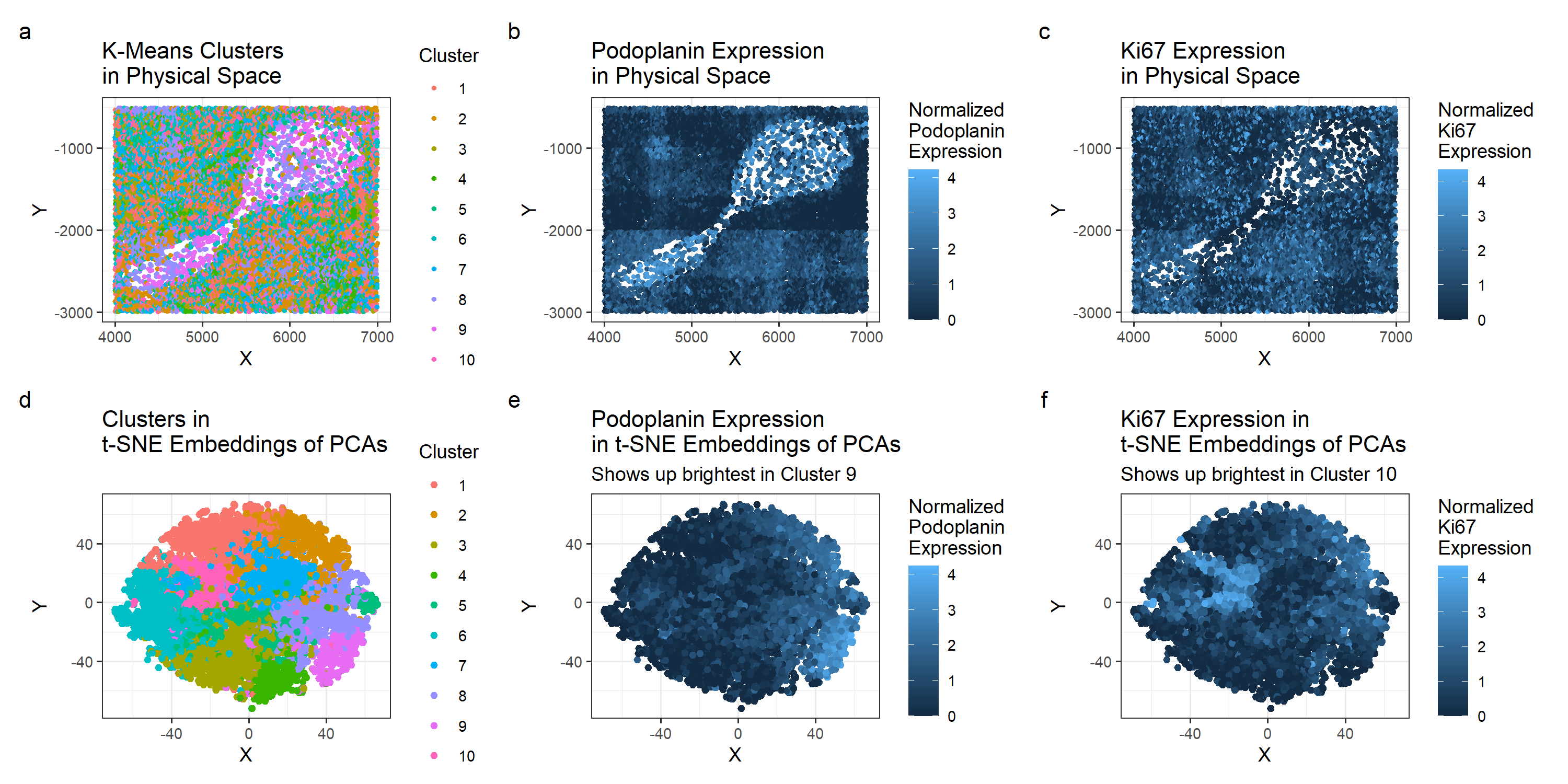
For this analysis, I normalized by gene expression and based on a withiness plot, chose 10 clusters for the k-means clustering. Figure A and D shows the clusters in physical space and in t-SNE embeddings of the PCA. Based on both visuals, Cluster 9 and Cluster 10 seemed to be the most interesting clusters to compare. In Figure A, they cover different areas within the tissue, with cluster 9 mainly concentrated in the sparse center and cluster 10 scattered in the denser outskirts. I performed a two-sided wilcox test for cluster 9 and cluster 10. Based on the calculated p-values and visualizations of gene expresssion, I chose to look at Podoplanin for cluster 9 and Ki67 for cluster 10. While they didn’t necessarily have the lowest p-value, they seemed to be the most contained within their respective cluster, making it more likely that they’re unique to the cell type represented by the said cluster.
Cluster 9: Podoplanin
A quick search for Podoplanin shows that it is “widely used as a marker for lymphatic endothelial cells and fibroblastic reticular cells of lymphoid organs” [1]. This suggests that cluster 9, with its high expression of Podoplanin, represents either one of these two cells. Additionally, it indicates that the tissue structure we’re working with is the white pulp. The white pulp is described by med.libretexts.org as tissue structure that “resembles the lymphoid follicles of the lymph” [2]. Based on this description and our observation of Podoplanin in cluster 9, it seems likely that this CODEX is of the white pulp. C l
Cluster 10: Ki-67
The Ki-67 at first didn’t seem to have a direct connection to a certain tissue structure. It seems mainly used to look at cell proliferation, which is useful when studying cancer [3]. However, it is not quite as useful for identifying regions of a spleen. The one use I saw connecting Ki-67 and the spleen is a paper that used to for identifying rapidly proliferating cells in the white pulp [4]. In the paper, Figure 2.F notes the high concentration of Ki-67 at the margins of the white pulp nodules and in a “small residiual reactive follicle center”. Based on the fact that Ki-67 is a marker for cell proliferation and on its use for looking at white pulp, it seems reasonable to conclude that cluster 10 is picking up on lymphoid follicles within the white pulp.
Conclusion: We have white pulp.
References
[1] https://www.ncbi.nlm.nih.gov/pmc/articles/PMC3439854/ [2] https://med.libretexts.org/Bookshelves/Anatomy_and_Physiology/Human_Anatomy_(OERI)/19%3A_Lymphatic_and_Immune_System/19.04%3A_Anatomy_of_Lymphatic_Organs_and_Tissues [3] https://onlinelibrary.wiley.com/doi/10.1002/(SICI)1097-4652(200003)182:3%3C311::AID-JCP1%3E3.0.CO;2-9 [4] https://www.sciencedirect.com/science/article/pii/S0006497120704921?ref=cra_js_challenge&fr=RR-1
Code
1
2
3
4
5
6
7
8
9
10
11
12
13
14
15
16
17
18
19
20
21
22
23
24
25
26
27
28
29
30
31
32
33
34
35
36
37
38
39
40
41
42
43
44
45
46
47
48
49
50
51
52
53
54
55
56
57
58
59
60
61
62
63
64
65
66
67
68
69
70
71
72
73
74
75
76
77
78
79
80
81
82
83
84
85
86
87
88
89
90
91
92
93
94
95
96
97
98
99
100
101
102
103
104
105
106
107
108
109
110
111
112
113
114
115
116
117
118
119
120
121
122
123
124
125
126
127
128
129
130
131
132
133
134
135
136
137
138
139
140
141
142
143
144
145
146
147
148
149
150
151
152
153
154
155
156
157
158
159
160
161
162
163
164
165
166
167
168
169
170
171
172
173
174
175
176
177
178
179
180
181
182
183
184
185
186
187
188
189
190
191
192
193
194
195
196
197
198
199
200
201
202
203
204
205
206
207
208
209
# hw6
data <- read.csv('C:\\Users\\emw\\OneDrive - Johns Hopkins\\spring 2024\\genomic-data-visualization-2024\\data\\codex_spleen_subset.csv.gz', row.names=1)
library(ggplot2)
library(patchwork)

#QUALITY CONTROL

#look at the data
colnames(data)
dim(data) # 11512    31
#split the data
pos <- data[, 1:2]
area <- data[, 3]
gexp <- data[4:ncol(data)]

#Plot Spatially
# Are there any areas with greater area?
df_physicalspace <- data.frame(data)
p_physicalspace_area <- ggplot(df_physicalspace) +
  geom_point(aes(x = x, y = y, col=area), size=1) +
  theme_bw() +
  labs(
    title = "Looking at Cell Area in Physical Space",
    x = "X",
    y = "Y", color="Area"
  )
df_physicalspace_gexp <- data.frame(pos=pos, gexp=gexp)
p_physicalspace_gexp <- ggplot(df_physicalspace_gexp) +
  geom_point(aes(x = pos.x, y = pos.y, col=rowSums(gexp)), size=1) +
  theme_bw() +
  labs(
    title = "Looking at the Total Gene Expression in Physical Space",
    x = "X",
    y = "Y", color="Total Gene\nExpression"
  )
p_physicalspace_area + p_physicalspace_gexp + plot_layout(ncol = 2) +plot_annotation(tag_levels = 'a')

# Doesn't seem to be a big difference, so just normalize by expression

#Normalize by Expression
gexpnorm <- log10(gexp/rowSums(gexp) * mean(rowSums(gexp))+1)

# CLUSTER

# Check withiness
withiness <- c(1:20)
for (i in 2:20) {
  kmeans_i <- kmeans(gexpnorm, centers = i)
  withiness[i] <- kmeans_i$tot.withinss
}
plot(x= c(2:20), y=withiness[2:20])

# there isn't a clear withiness, maybe 10?
set.seed(1)
com <- as.factor(kmeans(gexpnorm, centers=10)$cluster)
df <- data.frame(pos,gexpnorm, com)

# Looking at the clusters in physical space
df_physicalspace_com <- data.frame(pos=pos, cluster = com)
p_physicalspace_com <- ggplot(df_physicalspace_com) +
  geom_point(aes(x = pos.x, y = pos.y, col=cluster), size=1) +
  theme_bw() +
  labs(
    title = "K-Means Clusters \nin Physical Space",
    x = "X",
    y = "Y", color="Cluster"
  )
p_physicalspace_com


# DIMENSIONALITY REDUCTION
# PCA for Dataset
pcs_whole <- prcomp(df[, colnames(gexpnorm)])
dim(pcs_whole$x)
df2_whole <- data.frame(pcs_whole$x[,1:2])
p_pca_whole <- ggplot(df2_whole) + geom_point(aes(x = PC1, y = PC2, col = com)) + theme_classic()

## t-SNE
library(Rtsne)
emb1_whole <- Rtsne(pcs_whole$x[,1:15], dims = 2, perplexity = 5) ## what happens if we run tSNE on PCs?

df_whole <- data.frame(emb1_whole=emb1_whole$Y, cluster = com)
p_tsne_whole <- ggplot(df_whole) +
  geom_point(aes(x = emb1_whole.1, y = emb1_whole.2, col = com)) +
  theme_bw() +
  labs(
    title = "Clusters in \nt-SNE Embeddings of PCAs",
    x = "X",
    y = "Y", color="Cluster"
  )
p_tsne_whole

p_physicalspace_com + p_tsne_whole + plot_layout(ncol = 2) +plot_annotation(tag_levels = 'a')

# based on physical space, I want to compare cluster 9 10

# DIFFERENTIAL EXPRESSION ANALYSIS
# check each cluster for top performing genes
all_pvals_cluster9 <- c(length(colnames(gexpnorm)))
all_pvals_cluster10 <- c(length(colnames(gexpnorm)))
i <- 0
for (g in colnames(gexpnorm)) {
  i <- i+1
  p_value_9 <- (wilcox.test(gexpnorm[com == 9, g],
                          gexpnorm[com != 9, g],
                          alternative = "two.sided")$p.val)
  all_pvals_cluster9[i] <-p_value_9

  p_value_10 <- (wilcox.test(gexpnorm[com == 10, g],
                            gexpnorm[com != 10, g],
                            alternative = "two.sided")$p.val)
  all_pvals_cluster10[i] <-p_value_10

}

df_pvalues <- data.frame(gene_name = colnames(gexpnorm), pval_c9 = as.numeric(all_pvals_cluster9),pval_c10 = as.numeric(all_pvals_cluster10))

df_pvalues_sorted_c9 <- df_pvalues[order(df_pvalues$pval_c9), ]
df_pvalues_sorted_c9[1:10,]
#gene_name       pval_c9     pval_c10
#6     SMActin  0.000000e+00 2.269444e-01
#7  Podoplanin 3.083430e-286 1.194084e-16
#15       CD35 1.242972e-246 3.539619e-21
df_pvalues_sorted_c10 <- df_pvalues[order(df_pvalues$pval_c10), ]
df_pvalues_sorted_c10[1:10,]
#gene_name       pval_c9     pval_c10
#4        Ki67  7.456044e-36 0.000000e+00
#14      CD11c  7.566850e-17 3.137996e-46
#26       CD45  6.664124e-02 1.024245e-38


p_physicalspace_SMActin <- ggplot(df_physicalspace_gexp) +
  geom_point(aes(x = pos.x, y = pos.y, col=gexpnorm$SMActin)) +
  theme_bw() +
  labs(
    title = "SMActin Expression \nin Physical Space",
    x = "X",
    y = "Y", color="Normalized \nSMActin \nExpression"
  )

df_SMActin <- data.frame(emb1_whole=emb1_whole$Y, gene_exp=gexpnorm$SMActin)
p_tsne_SMActin <- ggplot(df_SMActin) +
  geom_point(aes(x = emb1_whole.1, y = emb1_whole.2, col = gene_exp)) +
  theme_bw() +
  labs(
    title = "SMActin Expression \nin t-SNE Embeddings of PCAs",
    subtitle = "Shows up brightest in Cluster 9, but also for 3 and 8.",
    x = "X",
    y = "Y", color="Normalized \nSMActin \nExpression"
  )

# Gene from Cluster 10
p_physicalspace_Ki67 <- ggplot(df_physicalspace_gexp) +
  geom_point(aes(x = pos.x, y = pos.y, col=gexpnorm$Ki67), size=1) +
  theme_bw() +
  labs(
    title = "Ki67 Expression \nin Physical Space",
    x = "X",
    y = "Y", color="Normalized \nKi67 \nExpression"
  )

df_Ki67 <- data.frame(emb1_whole=emb1_whole$Y, gene_exp=gexpnorm$Ki67)
p_tsne_Ki67 <- ggplot(df_Ki67) +
  geom_point(aes(x = emb1_whole.1, y = emb1_whole.2, col = gene_exp)) +
  theme_bw() +
  labs(
    title = "Ki67 Expression in \nt-SNE Embeddings of PCAs",
    subtitle = "Shows up brightest in Cluster 10",
    x = "X",
    y = "Y", color="Normalized \nKi67 \nExpression"
  )

p_physicalspace_Podoplanin <- ggplot(df_physicalspace_gexp) +
  geom_point(aes(x = pos.x, y = pos.y, col=gexpnorm$Podoplanin), size=1) +
  theme_bw() +
  labs(
    title = "Podoplanin Expression \nin Physical Space",
    x = "X",
    y = "Y", color="Normalized \nPodoplanin \nExpression"
  )

df_Podoplanin <- data.frame(emb1_whole=emb1_whole$Y, gene_exp=gexpnorm$Podoplanin)
p_tsne_Podoplanin <- ggplot(df_Podoplanin) +
  geom_point(aes(x = emb1_whole.1, y = emb1_whole.2, col = gene_exp)) +
  theme_bw() +
  labs(
    title = "Podoplanin Expression \nin t-SNE Embeddings of PCAs",
    subtitle = "Shows up brightest in Cluster 9",
    x = "X",
    y = "Y", color="Normalized \nPodoplanin \nExpression"
  )


# Best Gene for Cluster 9
p_tsne_Podoplanin

# Best Gene for Cluster 10
p_tsne_Ki67

# Mediocore Gene for Cluster 9, expresses too generally
p_tsne_SMActin

p_tsne_whole + p_tsne_SMActin + p_tsne_Podoplanin +p_tsne_Ki67+ plot_layout(ncol = 2) +plot_annotation(tag_levels = 'a')
p_physicalspace_com + p_physicalspace_SMActin + p_physicalspace_Podoplanin+ p_physicalspace_Ki67+plot_layout(ncol = 2) +plot_annotation(tag_levels = 'a')

# FINAL PLOT
p_physicalspace_com + p_physicalspace_Podoplanin+ p_physicalspace_Ki67+ p_tsne_whole +  p_tsne_Podoplanin +p_tsne_Ki67+plot_layout(ncol = 3) +plot_annotation(tag_levels = 'a')