Exploring Cell Types in CODEX Data

You will need to visualize and interpret at least two cell-types. Create a data visualization and write a description to convince me that your interpretation is correct.

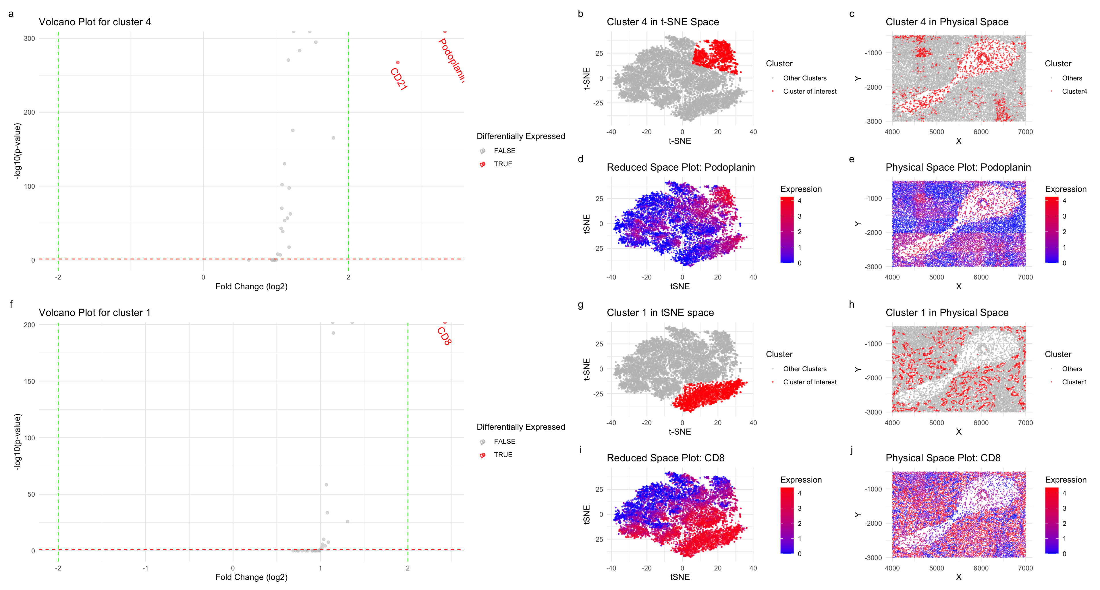
I started by first normalizing the dataset, and performed dimensionality reduction using tSNE. After finding an optimal k=6 value using the total withiness, I performed KMeans clustering. To further explore the cell types, I chose cluster 1, and 4. To perform the differential expression analysis, for both the cluster, I used wilcox-test and plotted the volcano plots taking into account p-values and a fold change greater than 2 or less than -2. Further, I plotted the expression level on tSNE and physical space.

Plots a-e correspond to cluster 4 analysis. For plots d,e I used color saturation to show the differences in the expression level in reduced and physical space. Location with higher expression levels in plot d,e corresponds to cluster 4’s coordinates in the reduced and physical space (b,c). Similar analysis was done for cluster 1 (plots f-j).

Your goal is to figure out what tissue structure is represented in the CODEX data. Options include: (1) Artery/Vein, (2) White pulp, (3) Red pulp, (4) Capsule/Trabecula

For cluster 4, I found that Podoplanin, and CD21 were differentially expressed. Podoplanin, is a protein, highly expressed in lymphatic endothelial cells and is involved in cell migration and adhesion [1]. CD21, a receptor found on mature B cells, follicular dendritic cells, and subsets of T cells and an important receptor for uptake and retention of immune complexes [2].The differential expression of these proteins suggests the presence of specialized cellular components within cluster 4, potentially corresponding to regions of germinal centers or lymphoid follicles.

Within cluster 1, differential expression of the CD8 protein was identified. CD8 is primarily expressed on cytotoxic T cells, which play a crucial role in the adaptive immune response by targeting and eliminating infected or abnormal cells. The presence of CD8-positive cells within cluster 1 suggests the involvement of cytotoxic T cells, which are typically found in proximity to antigen-presenting cells in lymphoid tissues [3]

Based on my analysis, the tissue structure represented in the CODEX data corresponds to at least white pulp, a distinctive region found within lymphoid organs such as the spleen [4]. There is also a possibility of the presence of artery/vein tissues due to the distinct cellular compositions they exhibit, including smooth muscle cells, endothelial cells, and pericytes, and I have explored only two clusters.

[1] Krishnan H, Rayes J, Miyashita T, et al. Podoplanin: An emerging cancer biomarker and therapeutic target. Cancer Sci. 2018;109(5):1292-1299. <doi:10.1111/cas.13580>
[2] https://www.sinobiological.com/resource/cd21/proteins
[3]Georg F. Weber, Harvey Cantor,CD8,Editor(s): Peter J. Delves, Encyclopedia of Immunology (Second Edition), Elsevier, 1998, Pages 475-478, ISBN 9780122267659, https://doi.org/10.1006/rwei.1999.0124. (https://www.sciencedirect.com/science/article/pii/B0122267656001298)
[4] https://training.seer.cancer.gov/anatomy/lymphatic/components/spleen.html

You must include the entire code you used to generate the figure so that it can be reproduced.

library(ggplot2)
library(patchwork)
library(Rtsne)
library(ggrepel)
data<-read.csv('/Users/nidhisoley/Desktop/GDataViz/codex_spleen_subset.csv.gz')
pos<-data[,2:3]
area<-data[,4]
pexp<-data[,5:32]
# plot x, y coord and visualize area

df<-data.frame(pos,area)
ggplot(df)+
  geom_point(aes(x=x,y=y,col=area),size=0.5)

pexpnorm <- log10(pexp/rowSums(pexp) * mean(rowSums(pexp))+1)
# perform pca
pcs <- prcomp(pexpnorm)

# run tsne on PCs
emb <- Rtsne(pcs$x)$Y

tot.witness = c()
for (i in 1:10){
  km <- kmeans(emb, centers=i)
  tot.witness = append(tot.witness, km$tot.withinss)
}
df.witness = data.frame(k=c(1:10), total.witness=tot.witness)
p<-ggplot(df.witness, aes(x=k, y=tot.witness)) + geom_line() + 
  geom_point() + theme_minimal() + scale_x_discrete(limits=as.factor(c(1:10)))
##kmeans
clusters <- as.factor(kmeans(emb, 6)$cluster)
p0<-ggplot(data.frame(emb,clusters))+geom_point(aes(x=X1,y=X2,col=clusters),size = 0.5, alpha=0.5)
###plot cluster in physical space
cluster1_of_interest<-4
df_physical <- data.frame(pos, Cluster = factor(clusters == cluster1_of_interest))
p1 <- ggplot(df_physical, aes(x = x, y = y, color = Cluster)) +
  geom_point(size = 0.2, alpha=0.5) +
  scale_color_manual(values = c("grey", "red"), labels = c("Others", "Cluster4")) +
  labs(
    x = "X",
    y = "Y",
    title = "Cluster 4 in Physical Space"
  ) +
  theme_minimal()
p1
# t-SNE Space Plot
df_tsne <- data.frame(emb, Cluster = factor(clusters == cluster1_of_interest))
p2 <- ggplot(df_tsne, aes(x = X1, y = X2, color = Cluster)) +
  geom_point(size = 0.5, alpha=0.5) +
  scale_color_manual(values = c("grey", "red"), labels = c("Other Clusters", "Cluster of Interest")) +
  labs(
    x = "t-SNE",
    y = "t-SNE",
    title = "Cluster 4 in t-SNE Space"
  ) +
  theme_minimal()
p2
###genes in cluster 4
pvals <- sapply(colnames(pexpnorm), function(p) {
  test <- wilcox.test(pexpnorm[clusters == cluster1_of_interest, p], 
                      pexpnorm[clusters != cluster1_of_interest, p], alternative = 'greater')
  test$p.value
})

fc <- sapply(colnames(pexpnorm), function(p) {
  mean(pexpnorm[clusters == cluster1_of_interest, p]) / mean(pexpnorm[clusters != cluster1_of_interest, p])
})

volcano_data <- data.frame(pvals = pvals, fc = fc, label = colnames(pexpnorm))

top_upregulated <- volcano_data[volcano_data$fc > 2 & volcano_data$pvals < 0.05, "label"]
top_downregulated <- volcano_data[volcano_data$fc < -2 & volcano_data$pvals < 0.05, "label"]

p3 <- ggplot(volcano_data, aes(x = fc, y = -log10(pvals), color = factor(label %in% c(top_upregulated, top_downregulated)))) +
  geom_point(alpha = 0.5) +
  scale_color_manual(values = c("gray", "red", "blue")) +
  geom_hline(yintercept = -log10(0.05), linetype = "dashed", color = "red") +
  geom_vline(xintercept = c(-2, 2), linetype = "dashed", color = "green") +
  labs(
    title = "Volcano Plot for cluster 4",
    x = "Fold Change (log2)",
    y = "-log10(p-value)",
    color = "Differentially Expressed"
  ) +
  geom_text(aes(label = ifelse(label %in% c(top_upregulated, top_downregulated), label, "")), size=4.5, hjust=-0.1, vjust=1.5,
            angle=300) +
  theme_minimal()

p3

###podoplanin physical and reduce space
gene1_of_interest <- "Podoplanin"
expression_levels <- pexpnorm[, gene1_of_interest]
plot_data <- data.frame(emb, Expression = expression_levels)

p4 <- ggplot(plot_data, aes(x = X1, y = X2)) +
  geom_point(aes(color = Expression), size = 0.3, alpha=0.5) +  
  scale_color_gradient(low = "blue", high = "red") +  
  labs(
    x = "tSNE",
    y = "tSNE",
    title = paste("Reduced Space Plot:", gene1_of_interest)
  ) +
  theme_minimal()

plot_data <- data.frame(pos, Expression = expression_levels)
p5 <- ggplot(plot_data, aes(x = x, y = y)) +
  geom_point(aes(color = Expression), size = 0.1, alpha=0.5) +  
  scale_color_gradient(low = "blue", high = "red") +  
  labs(
    x = "X",
    y = "Y",
    title = paste("Physical Space Plot:", gene1_of_interest)
  ) +
  theme_minimal()
p5

##cluster change:1

###plot cluster in physical space
cluster2_of_interest<-1
df_physical <- data.frame(pos, Cluster = factor(clusters == cluster2_of_interest))
p1.2 <- ggplot(df_physical, aes(x = x, y = y, color = Cluster)) +
  geom_point(size = 0.2, alpha=0.5) +
  scale_color_manual(values = c("grey", "red"), labels = c("Others", "Cluster1")) +
  labs(
    x = "X",
    y = "Y",
    title = "Cluster 1 in Physical Space"
  ) +
  theme_minimal()
p1.2
# t-SNE Space Plot
df_tsne <- data.frame(emb, Cluster = factor(clusters == cluster2_of_interest))
p2.2 <- ggplot(df_tsne, aes(x = X1, y = X2, color = Cluster)) +
  geom_point(size = 0.5, alpha=0.5) +
  scale_color_manual(values = c("grey", "red"), labels = c("Other Clusters", "Cluster of Interest")) +
  labs(
    x = "t-SNE",
    y = "t-SNE",
    title = "Cluster 1 in tSNE space"
  ) +
  theme_minimal()
p2.2


###genes in cluster 4
pvals_2 <- sapply(colnames(pexpnorm), function(p) {
  test <- wilcox.test(pexpnorm[clusters == cluster2_of_interest, p], 
                      pexpnorm[clusters != cluster2_of_interest, p], alternative = 'greater')
  test$p.value
})

fc_2 <- sapply(colnames(pexpnorm), function(p) {
  mean(pexpnorm[clusters == cluster2_of_interest, p]) / mean(pexpnorm[clusters != cluster2_of_interest, p])
})

volcano_data_2 <- data.frame(pvals = pvals_2, fc = fc_2, label = colnames(pexpnorm))

top_upregulated_2<- volcano_data_2[volcano_data_2$fc> 2 & volcano_data_2$pvals < 0.05, "label"]
top_downregulated_2 <- volcano_data_2[volcano_data_2$fc < -2 & volcano_data_2$pvals < 0.05, "label"]

p3.2 <- ggplot(volcano_data_2, aes(x = fc, y = -log10(pvals), color = factor(label %in% c(top_upregulated_2, top_downregulated_2)))) +
  geom_point(alpha = 0.5) +
  scale_color_manual(values = c("gray", "red", "blue")) +
  geom_hline(yintercept = -log10(0.05), linetype = "dashed", color = "red") +
  geom_vline(xintercept = c(-2, 2), linetype = "dashed", color = "green") +
  labs(
    title = "Volcano Plot for cluster 1",
    x = "Fold Change (log2)",
    y = "-log10(p-value)",
    color = "Differentially Expressed"
  ) +
  geom_text(aes(label = ifelse(label %in% c(top_upregulated_2, top_downregulated_2), label, "")), size=4.5, hjust=-0.1, vjust=1.5,
            angle=300) +
  theme_minimal()

p3.2

###podoplanin physical and reduce space
gene2_of_interest <- "CD8"
expression_levels <- pexpnorm[, gene2_of_interest]

plot_data <- data.frame(emb, Expression = expression_levels)

p4.2 <- ggplot(plot_data, aes(x = X1, y = X2)) +
  geom_point(aes(color = Expression), size = 0.4, alpha=0.5) + 
  scale_color_gradient(low = "blue", high = "red") +  
  labs(
    x = "tSNE",
    y = "tSNE",
    title = paste("Reduced Space Plot:", gene2_of_interest)
  ) +
  theme_minimal()
p4.2
plot_data <- data.frame(pos, Expression = expression_levels)
p5.2 <- ggplot(plot_data, aes(x = x, y = y)) +
  geom_point(aes(color = Expression), size = 0.05,alpha=0.5) +  
  scale_color_gradient(low = "blue", high = "red") +  
  labs(
    x = "X",
    y = "Y",
    title = paste("Physical Space Plot:", gene2_of_interest)
  ) +
  theme_minimal()
p5.2

(p3 + (p2 + p1 + p4 + p5 + ncol(2))) / (p3.2 + (p2.2 + p1.2 + p4.2 + p5.2 + ncol(2)))+plot_annotation(tag_levels = 'a')