Cell Cluster Identification and Validation in Breast Tumor Tissue

###Cluster of interest 1 (cluster 5)
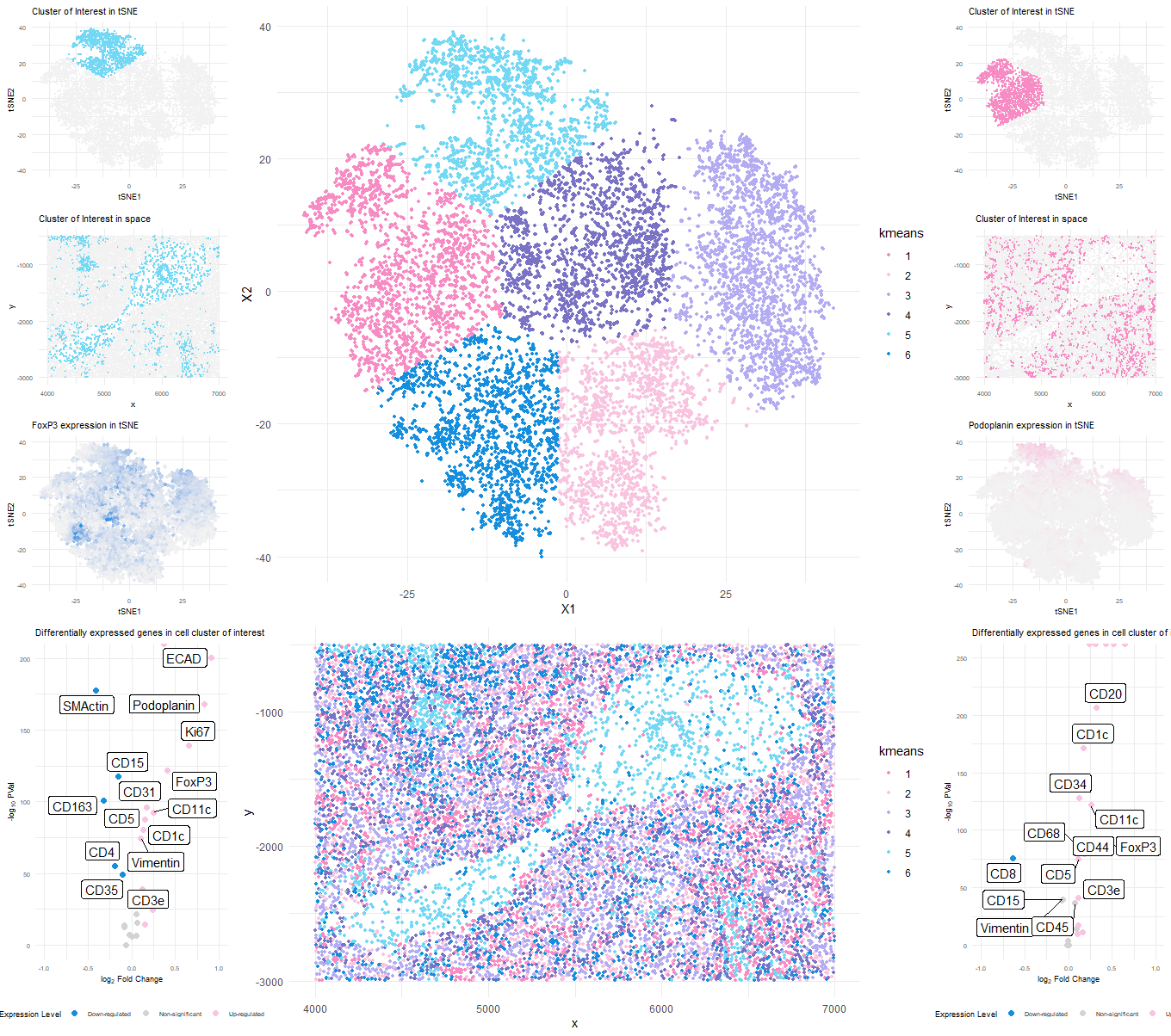
Based on the upregulated markers in the volcano plot it seems like the cell cluster could be representing Artery/Vein tissue structure.
-
CD31 (PECAM-1): CD31 is commonly used as a marker for endothelial cells, which line the interior surface of blood vessels, including arteries and veins[1].
-
Ki67: This is a nuclear protein associated with cell proliferation[2]. Its presence suggests active cell division, which could be seen in various tissues, including blood vessels during angiogenesis [1].
-
ECAD (E-Cadherin): This is a marker for epithelial cells, which could be present in the endothelium of blood vessels [1].
-
FoxP3: This is a transcription factor that is a master regulator for the development and function of regulatory T cells3. Its presence suggests the involvement of regulatory T cells [3].
-
Collagen IV: This is a type of collagen found primarily in the basal lamina, a layer of the extracellular matrix of many tissues, including blood vessels [1].
###Cluster of interest 2 (cluster 2)
It seems like the cell cluster might be more related to White Pulp which is a part of the spleen containing mostly immune cells including T cells, B cells, and macrophages.
Given the presence of hematopoietic stem cell markers (CD34), dendritic cell markers (CD1c, CD11c), T regulatory cell marker (FoxP3), and a marker for histiocytes (CD68), it suggests a high likelihood of immune cell involvement. The presence of ECAD indicates epithelial cells, and CD44 is associated with cancer stem cells.
-
Podoplanin: This is a marker for lymphatic endothelial cells[1].
-
CD34: This is a marker of hematopoietic stem cells¹. It’s also a marker of vascular endothelial cells [4].
-
ECAD (E-Cadherin): It’s a transmembrane protein involved in cellular adhesion and polarity maintenance. It’s expressed in almost all epithelial cells [4][5].
-
CD1c: This is a defined marker of subsets of conventional dendritic cells [6]. CD11c: It’s a widely recognized dendritic cell marker [7].
-
FoxP3: This is a specific marker of natural T regulatory cells and adaptive/induced T regulatory cells [8].
-
CD68: It’s a lysosomal glycoprotein primarily used as a marker to identify histiocytes and histiocytic tumors [9].
References
[1] “Cell Markers Explained.” Boster Bio. Accessed April 22, 2024. https://www.bosterbio.com/protocols-and-troubleshooting/tips/cell-markers-explained [2] Sakaguchi, S., Miyara, M., Costantino, C. M., & Hafler, D. A. (2010). FOXP3+ regulatory T cells in the human immune system. Nature Reviews Immunology, 10(7), 490-500. doi:10.1038/nri2785 [3] Gerdes, J., Lemke, H., Baisch, H., Wacker, H. H., Schwab, U., & Stein, H. (1984). Cell cycle analysis of a cell proliferation-associated human nuclear antigen defined by the monoclonal antibody Ki-67. Journal of Immunology, 133(4), 1710-1715. PMID: 6206131 [4] Anjos-Afonso, F., & Bonnet, D. (2023). Human CD34+ hematopoietic stem cell hierarchy: how far are we with its delineation at the most primitive level? Blood, 142(6), 509–518 [5] Bidot, S., & Li, X. (2024). E-cadherin. PathologyOutlines.com. Retrieved February 19, 2024, from PathologyOutlines.com website. [6] OriGene Technologies, Inc. (n.d.). CD1C: A Dendritic Cell Surface Marker that Induces T-Cell. Retrieved February 22, 2024, from OriGene website [7] NeoBiotechnologies. (2023). Cheat Sheet to CD11c: Dendritic Cell Marker Explained. Retrieved February 22, 2024, from NeoBiotechnologies website. [8] “FoxP3.” Wikipedia. https://en.wikipedia.org/wiki/FoxP3 [9] “CD68.” Wikipedia. https://en.wikipedia.org/wiki/CD68
Source Code
data <- read.csv("C:/Users/ivych/OneDrive - Johns Hopkins/Classes/Data Visualization/codex_spleen_subset.csv.gz",row.names = 1)
# install.packages("viridisLite")

library(viridis)
library(ggplot2)
library(gridExtra)

head(data)
dim(data)

xiao_plt <- c(
  "#f78bc4",
  "#f8c4e0",
  "#b3acf2",
  "#7a72c5",
  "#72d8f4",
  "#158edd")

pos <- data[,1:2]
area <- data[,3]

gexp <-data[,4:ncol(data)]
gexp[1:5, 1:5]
hist(rowSums(gexp))


#normalization
mat <- log10(gexp/rowSums(gexp) * mean(rowSums(gexp))+1)
hist(log(mat[,'CD4'])+1)

#tSNE
emb <-  Rtsne::Rtsne(mat)$Y

#scree plot
ks <-1:15
k_out <- do.call(rbind, lapply(ks,function(g){
  com <- kmeans(emb, centers=g)
  c(within = com$tot.withiness, between=com$betweenss)
}))

plot(ks, -(k_out[,1]),type='l')

k = 6 # decided k
com<-kmeans(emb, centers=k)
df1 <- data.frame(emb, kmeans=as.factor(com$cluster))
p_kmeans = ggplot(df1) +
  geom_point(aes(x=X1, y=X2, col=kmeans),
              size=1,alpha=1) + theme_minimal() +
  scale_colour_manual(values = xiao_plt)
p_kmeans

df2 <- data.frame(data, kmeans=as.factor(com$cluster))
head(df)
p_kmeans2 = ggplot(df2) +
  geom_point(aes(x=x, y=y, col=kmeans),
              size=1, alpha=1) + theme_minimal()+
  scale_colour_manual(values = xiao_plt)
p_kmeans2


# pick cluster of interest
coi <- 5

#cluster of interest in the tsne space
p_c1 <- ggplot(df1) +
  geom_point(size = 0.5,aes(x = X1, y = X2, col=(kmeans==coi))) +
  labs(title = 'Cluster of Interest in tSNE',
       x = 'tSNE1', y = 'tSNE2',col="in cluster 2") +
  theme_minimal() + theme(legend.position = "none") +
  scale_colour_manual(values = c("grey95",xiao_plt[coi])) + theme(text = element_text(size=7))
p_c1

#cluster of interest in the physical space
p_c2 <- ggplot(df2) +
  geom_point(size = 0.5, aes(x = x, y = y, col=(kmeans==coi))) +
  labs(title = 'Cluster of Interest in space',
       x = 'x', y = 'y',col="Cell in cluster 2") +
  theme_minimal() + theme(legend.position = "none", legend.key.size = unit(1, "cm")) +
  scale_colour_manual(values = c("grey95",xiao_plt[coi]))+ theme(text = element_text(size=7))
p_c2


## Double-sided wilcox test to identify differential expression
km_c = as.factor(com$cluster)
cluster.oi<- names(which(df2$kmeans == coi))
cluster.ot <- names(which(df2$kmeans != coi))

#differential genes
pvs<- sapply(colnames(gexp), function(g) {
  wilcox.test(mat[km_c == coi, g],
                      mat[km_c != coi, g],)$p.val
})

names(which(pvs < 1e-8))
head(sort(pvs), n=20)


#fold change
log2fc <- sapply(colnames(gexp), function(f) {
  log2(mean(mat[km_c == coi, f])/mean(mat[km_c != coi, f]))
})


#volcano plot
df_volcano <- data.frame(pvs, log2fc)
exp_sig <- apply(df_volcano, 1, function(g) {
  if (g[2] >= 0.1 & g[1] <= 0.05) {out = "Up-regulated"}
  else if (g[2] <= -0.1 & g[1] <= 0.05) {out = "Down-regulated"}
  else {out = "Non-significant"}
  out})
data_deg <- cbind(df_volcano, exp_sig)


p_volc <- ggplot(data_deg, aes(y=-log10(pvs), x=log2fc)) +
  scale_color_manual(values = c(xiao_plt[6], "lightgray", xiao_plt[2])) +
  geom_point(aes(col = exp_sig),size=2) +
  ggrepel::geom_label_repel(label=rownames(data_deg)) +
  xlab(expression("log"[2]*" Fold Change")) +
  ylab(expression("-log"[10]*" PVal")) +
  theme_minimal()+
  theme(legend.position = 'bottom') +
  labs(title = 'Differentially expressed genes in cell cluster of interest',
       col = "Expression Level") +
  xlim(-1, 1)+ theme(text = element_text(size=7))
p_volc


# pick cluster of interest
coi2 <- 1

#cluster of interest in the tsne space
p_c1_2 <- ggplot(df1) +
  geom_point(size = 0.5,aes(x = X1, y = X2, col=(kmeans==coi2))) +
  labs(title = 'Cluster of Interest in tSNE',
       x = 'tSNE1', y = 'tSNE2',col="in cluster 2") +
  theme_minimal() + theme(legend.position = "none") +
  scale_colour_manual(values = c("grey95",xiao_plt[coi2]))+ theme(text = element_text(size=7))
p_c1_2

#cluster of interest in the physical space
p_c2_2 <- ggplot(df2) +
  geom_point(size = 0.5, aes(x = x, y = y, col=(kmeans==coi2))) +
  labs(title = 'Cluster of Interest in space',
       x = 'x', y = 'y',col="Cell in cluster 2") +
  theme_minimal() + theme(legend.position = "none", legend.key.size = unit(1, "cm")) +
  scale_colour_manual(values = c("grey95",xiao_plt[coi2]))+ theme(text = element_text(size=7))
p_c2_2


## Double-sided wilcox test to identify differential expression
km_c2 = as.factor(com$cluster)

#differential genes
pvs2<- sapply(colnames(gexp), function(g) {
  wilcox.test(mat[km_c2 == coi2, g],
              mat[km_c2 != coi2, g],)$p.val
})

names(which(pvs2 < 1e-8))
head(sort(pvs2), n=20)


#fold change
log2fc2 <- sapply(colnames(gexp), function(f) {
  log2(mean(mat[km_c2 == coi2, f])/mean(mat[km_c2 != coi2, f]))
})


#volcano plot
df_volcano2 <- data.frame(pvs2, log2fc2)
exp_sig2 <- apply(df_volcano2, 1, function(g) {
  if (g[2] >= 0.1 & g[1] <= 0.05) {out = "Up-regulated"}
  else if (g[2] <= -0.1 & g[1] <= 0.05) {out = "Down-regulated"}
  else {out = "Non-significant"}
  out})
data_deg2 <- cbind(df_volcano2, exp_sig2)


p_volc_2 <- ggplot(data_deg2, aes(y=-log10(pvs2), x=log2fc2)) +
  scale_color_manual(values = c(xiao_plt[6], "lightgray", xiao_plt[2])) +
  geom_point(aes(col = exp_sig2),size=2) +
  ggrepel::geom_label_repel(label=rownames(data_deg2)) +
  xlab(expression("log"[2]*" Fold Change")) +
  ylab(expression("-log"[10]*" PVal")) +
  theme_minimal()+
  theme(legend.position = 'bottom') +
  labs(title = 'Differentially expressed genes in cell cluster of interest 2',
       col = "Expression Level") +
  xlim(-1, 1) + ylim(0,250)+ theme(text = element_text(size=7))
p_volc_2


df_FoxP3 <- cbind(df1,FoxP3 = mat$FoxP3)

p_FoxP3 <- ggplot(df_FoxP3) +
  geom_point(size = 1,aes(x = X1, y = X2, col = FoxP3^2)) +
  theme_minimal()+ theme(legend.position="none", legend.key.size = unit(0.2, "cm")) +
  labs(title = 'FoxP3 expression in tSNE',
       x = 'tSNE1', y = 'tSNE2') +
  scale_color_gradient(low = 'grey95', high=xiao_plt[6]) + theme(text = element_text(size=7))
p_FoxP3

df_Podoplanin <- cbind(df1,Podoplanin = mat$Podoplanin)

p_Podoplanin <- ggplot(df_Podoplanin) +
  geom_point(size = 1,aes(x = X1, y = X2, col = Podoplanin^2)) +
  theme_minimal()+ theme(legend.position="none", legend.key.size = unit(0.2, "cm")) +
  labs(title = 'Podoplanin expression in tSNE',
       x = 'tSNE1', y = 'tSNE2') +
  scale_color_gradient(low = 'grey95', high=xiao_plt[2]) + theme(text = element_text(size=7))
p_Podoplanin

#plot panel arrangement
layout <- rbind(c(3,1,1,1,6),
                c(4,1,1,1,7),
                c(9,1,1,1,10),
                c(5,2,2,2,8),
                c(5,2,2,2,8))
grid.arrange(p_kmeans,p_kmeans2,
             p_c1,p_c2,p_volc,
             p_c1_2,p_c2_2,p_volc_2,
             p_FoxP3,p_Podoplanin,
             layout_matrix = layout)