Visualizing Cells in CODEX to Identify Tissue Structure

Interpret the tissue structure in CODEX DATA

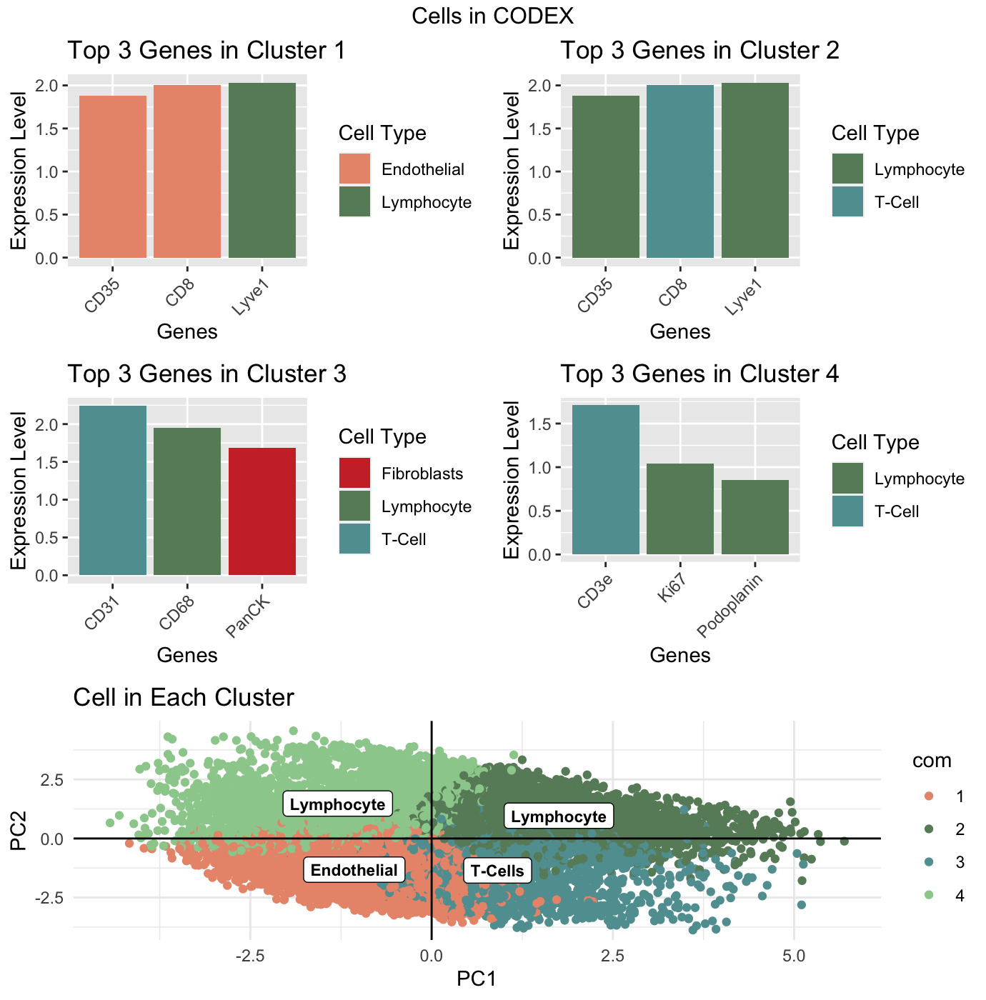
I performed principle component analysis on the normalized data and then used a withiness test to find that the data should be split into 4 clusters. I then plotted these clusters and perfermed a wilcox test on each one to get the top 3 differentially expressed genes in each clsuter. I identifyed the cell-type each gene is generally upregulated in and plotted the expression of the top 3 genes for each cluster in their own bar graphs. These bar graphs also identified the cell-type of each gene by color. Finally, I identified the most common cell-type of each clsuter based on the bar graphs and labeled each cluster as primarily containing cells of that type.

As can be seen by the k-means plot, both clusters 2 and 4 predominantly contained lymphocytes and cluster 3 more specifically contained T-cells, a type of lymphocytes. From the the bar graphs, we can see that the last cluster: clusters 1, also contained differentially expressed genes found in lymphocytes. As such, I believe this dataset contains lymphocytes, and according to a NIH article on the Histopathology of the Spleen, lymphocytes are primarily found in the white pulp of the spleen. Therefore, the CODEX dataset is representing the white pulp tissue structure in the spleen.

External Source: Cells identified from genes: https://www.proteinatlas.org Tissue structure identified from cell-type: https://www.ncbi.nlm.nih.gov/pmc/articles/PMC1828535/

The entire code used to generate the figure so that it can be reproduced.

library(ggplot2)
library(Rtsne)
library(patchwork)
library(gganimate)
library(lattice)
library(ggrepel)

data <- read.csv('/Users/shailitripathi/genomic-data-visualization-2024/data/codex_spleen_subset.csv.gz', row.names=1)

head(data)
data[1:5, 1:9] # intensity of each protein in a given area
dim(data) #11,512 cells and 28 proteins (31 - x, y, area)

pos <- data[, 1:2]
area <- data[, 3]
pexp <- data[, 4:31]

# Normalize
pexpnorm <- log10(pexp/rowSums(pexp) * mean(rowSums(pexp)) + 1)

# PCA 
pcs <- prcomp(pexpnorm)
plot(pcs$sdev[1:30], type = 'l') # plot variance of first 30 pcs
pc_plot <- ggplot(data.frame(pcs$x)) + geom_point(aes(x = PC1, y = PC2)) +
  geom_hline(yintercept = 0, linetype = "solid", color = "black") +
  geom_vline(xintercept = 0, linetype = "solid", color = "black") + 
  theme_minimal() 
pc_plot

# tSNE
emb <- Rtsne(pcs$x[, 1:5])$Y # 5 pcs 
ggplot(data.frame(emb)) + geom_point(aes(x = X1, y = X2))

# k-means clustering
set.seed(123)

totw <- sapply(1:10, function(i) {
  com <- kmeans(pcs$x[, 1:5], centers = i)
  return(com$tot.withinss)
})
plot(totw, type = 'l')

com <- kmeans(pcs$x[, 1:5], centers = 4)
cluster_labels <- as.factor(com$cluster)

pca_cluster <- ggplot(data.frame(pcs$x[, 1:2], com = cluster_labels)) +
  geom_point(aes(x = PC1, y = PC2, col = com)) +
  labs(title = "Clusters in PCA Space") + 
  geom_hline(yintercept = 0, linetype = "solid", color = "black") +
  geom_vline(xintercept = 0, linetype = "solid", color = "black") + 
  theme_minimal() 
pca_cluster


actual_cluster <- ggplot(data.frame(pos, com = cluster_labels)) +
  geom_point(aes(x = x, y = y, col = com)) +
  labs(title = "Clusters in Actual Space") 

pca_cluster + actual_cluster

# Clusters of Interest
names(sort(apply(pexp, 2, var), decreasing=TRUE)[1:10])
names(sort(apply(pexp, 2, mean), decreasing=TRUE)[1:10])

cl <- as.factor(com$cluster)
top_genes <- list()

for (cluster_id in unique(cl)) {
  dif_exp <- sapply(colnames(pexpnorm), function(gene){
    wilcox.test(pexpnorm[cl == cluster_id, gene], pexpnorm[cl != cluster_id, gene])$p.val
  })
  top_genes[[paste0("Cluster_", cluster_id)]] <- names(sort(dif_exp, decreasing = FALSE))[1:3]
}
top_genes

# Cluster 4 
top_genes_cluster_4 <- top_genes[["Cluster_4"]]
cell_types <- c("Lymphocyte", "T-Cell", "Lymphocyte")

top_genes_expression <- pexpnorm[, top_genes_cluster_4]
plot_data <- data.frame(Gene = top_genes_cluster_4, 
                        Expression = colMeans(top_genes_expression),
                        Cell_Type = cell_types)

cl4 <- ggplot(plot_data, aes(x = Gene, y = Expression, fill = Cell_Type)) +
  geom_bar(stat = "identity") +
  labs(title = "Top 3 Genes in Cluster 4",
       x = "Genes", y = "Expression Level", fill = "Cell Type") +
  theme(axis.text.x = element_text(angle = 45, hjust = 1)) +
  scale_fill_manual(values = c("Lymphocyte" = "darkseagreen4", "T-Cell" = "cadetblue"))
cl4

# Cluster 3
top_genes_cluster_3 <- top_genes[["Cluster_3"]]
cell_types <- c("T-Cell", "Lymphocyte", "Fibroblasts")

top_genes_expression <- pexpnorm[, top_genes_cluster_3]
plot_data <- data.frame(Gene = top_genes_cluster_3, 
                        Expression = colMeans(top_genes_expression),
                        Cell_Type = cell_types)

cl3 <- ggplot(plot_data, aes(x = Gene, y = Expression, fill = Cell_Type)) +
  geom_bar(stat = "identity") +
  labs(title = "Top 3 Genes in Cluster 3",
       x = "Genes", y = "Expression Level", fill = "Cell Type") +
  theme(axis.text.x = element_text(angle = 45, hjust = 1)) +
  scale_fill_manual(values = c("Lymphocyte" = "darkseagreen4", "T-Cell" = "cadetblue", "Fibroblasts" = "brown3"))
cl3

# Cluster 2
top_genes_cluster_2 <- top_genes[["Cluster_2"]]
cell_types <- c("T-Cell", "Lymphocyte", "Lymphocyte")

top_genes_expression <- pexpnorm[, top_genes_cluster_2]
plot_data <- data.frame(Gene = top_genes_cluster_2, 
                        Expression = colMeans(top_genes_expression),
                        Cell_Type = cell_types)

cl2 <- ggplot(plot_data, aes(x = Gene, y = Expression, fill = Cell_Type)) +
  geom_bar(stat = "identity") +
  labs(title = "Top 3 Genes in Cluster 2",
       x = "Genes", y = "Expression Level", fill = "Cell Type") +
  theme(axis.text.x = element_text(angle = 45, hjust = 1)) +
  scale_fill_manual(values = c("Lymphocyte" = "darkseagreen4", "T-Cell" = "cadetblue"))

# Cluster 1
top_genes_cluster_1 <- top_genes[["Cluster_1"]]
cell_types <- c("Endothelial", "Lymphocyte", "Endothelial")

top_genes_expression <- pexpnorm[, top_genes_cluster_2]
plot_data <- data.frame(Gene = top_genes_cluster_2, 
                        Expression = colMeans(top_genes_expression),
                        Cell_Type = cell_types)

cl1 <- ggplot(plot_data, aes(x = Gene, y = Expression, fill = Cell_Type)) +
  geom_bar(stat = "identity") +
  labs(title = "Top 3 Genes in Cluster 1",
       x = "Genes", y = "Expression Level", fill = "Cell Type") +
  theme(axis.text.x = element_text(angle = 45, hjust = 1)) +
  scale_fill_manual(values = c("Lymphocyte" = "darkseagreen4", "Endothelial" = "darksalmon"))

bars_of_clusters <- cl1 + cl2 + cl3 + cl4



cluster_tags <- c("Endothelial", "Lymphocyte", "T-Cells", "Lymphocyte")
cluster_colors <- c("darksalmon", "darkseagreen4", "cadetblue", "darkseagreen3")

pca_cluster <- ggplot(data.frame(pcs$x[, 1:2], com = cluster_labels)) +
  geom_point(aes(x = PC1, y = PC2, col = com)) +
  scale_color_manual(values = cluster_colors) +  
  labs(title = "Cell in Each Cluster") + 
  geom_hline(yintercept = 0, linetype = "solid", color = "black") +
  geom_vline(xintercept = 0, linetype = "solid", color = "black") + 
  theme_minimal()

tags_df <- data.frame(
  tag = cluster_tags,
  PC1 = tapply(pcs$x[, 1], cluster_labels, mean),
  PC2 = tapply(pcs$x[, 2], cluster_labels, mean)
)

cells_of_clusters <- pca_cluster +
  geom_label(data = tags_df, aes(label = tag, x = PC1, y = PC2), 
             color = "black", fill = "white", size = 3, fontface = "bold", vjust = 0.5)


# Combine Plots
bars_of_clusters <- cl1 + cl2 + cl3 + cl4
bars_of_clusters + cells_of_clusters

lay <- rbind(c(1,2),
             c(3,4),
             c(5,5))

grid.arrange(cl1, cl2,
             cl3, cl4,
             cells_of_clusters,
             layout_matrix = lay,
             top = "Cells in CODEX")