characterizing spatial gene expression heterogeneity in spatially resolved single-cell transcriptomics data with nonuniform cellular densities
In order to cluster genes that mark similar spatial patterns in space as well as infer evidence of cellular communication between spatially co-localized cell-types, MERINGUE computes a spatial cross-correlation statistic. In this tutorial, we will explore the distinction between this spatial cross-correlation statistic compared to a general (spatially-unaware) cross-correlation using simulations.
suppressMessages(library(MERINGUE))
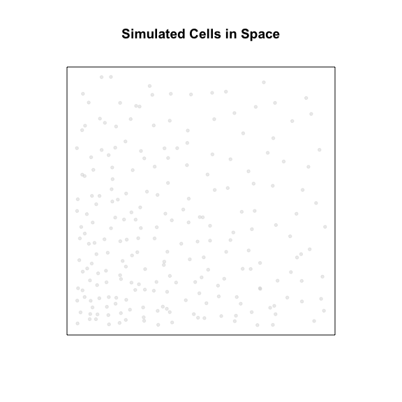
Simulate cells in space
First, let’s simulate some cells in space. Each point here is a cell. Their location in the plot can be interpreted as their physical location in space.
# 15x15 grid of cells
N <- 15^2
pos <- t(combn(c(1:sqrt(N), rev(1:sqrt(N))), 2))
pos <- unique(pos)
rownames(pos) <- paste0('cell', 1:N)
colnames(pos) <- c('x', 'y')
# jitter
posj <- jitter(pos, amount = 0.5)
# induce warping
posw <- 1.1^posj
# plot
par(mfrow=c(1,1), mar=rep(5,4))
plotEmbedding(posw,  main='Simulated Cells in Space')
Next, let’s simulate various gene expression patterns to highlight different scenarios that will help highlight the distinction spatial cross-correlation versus general (spatially-unaware) cross-correlation.
Scenario 1: General cross-correlation and spatial cross-correlation suggest similar trends
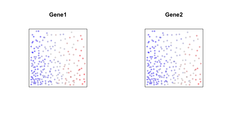
First, let’s consider two genes, Gene1 and Gene2. Both genes are
expressed in all cells but along a gradient. Cells spatially located
towards the left will generally have higher expression of Gene1 and
also higher expression of Gene2 compared to cells on the right. We can
visualize these gradients by coloring cells based on their expression
levels of the two genes.
par(mfrow=c(1,2), mar=rep(5,4))
gexp0 <- sort(abs(rnorm(N)))

set.seed(0)
gexp1 <- jitter(gexp0, amount = 0.5)
names(gexp1) <- rownames(pos)
plotEmbedding(posw, col=gexp1,
              main='Gene1')

set.seed(1)
gexp2 <- jitter(gexp0, amount = 0.5)
names(gexp2) <- rownames(pos)
plotEmbedding(posw, col=gexp2,
              main='Gene2')
If we plot the expression of Gene1 versus Gene2, as expected, we see
a positive relationship. Likewise, if we compute a general
cross-correlation statistic between Gene1 and Gene2, we can identify
a significant positive cross-correlation - that is, cells that express
higher levels of Gene1 tend to express higher levels of Gene2 and
cells that express lower levels of Gene1 tend to express lower levels
of Gene2.
# Plot
par(mfrow=c(1,1), mar=rep(5,4))
plot(gexp1, gexp2,
     main='Scatterplot of\nGene1 versus Gene2')
abline(lm(gexp2~gexp1))
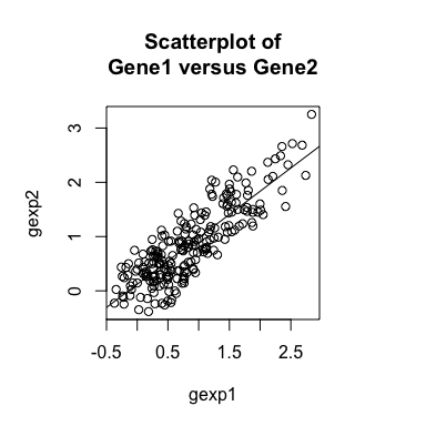
# Compute cross correlation
cor.test(gexp1, gexp2)

##
##  Pearson's product-moment correlation
##
## data:  gexp1 and gexp2
## t = 23.877, df = 223, p-value < 2.2e-16
## alternative hypothesis: true correlation is not equal to 0
## 95 percent confidence interval:
##  0.8064783 0.8809425
## sample estimates:
##      cor
## 0.847839
Likewise, if we compute a spatial cross-correlation statistic between
Gene1 and Gene2, we can identify a significant positive spatial
cross-correlation - that is, cells that express higher levels of Gene1
tend to be spatially neighboring cells that tend to express higher
levels of Gene2 and cells that express lower levels of Gene1 tend to
be spatially neighboring cells that tend to express lower levels of
Gene2.
weight <- getSpatialNeighbors(posw, filterDist = 1)
plotNetwork(posw, weight)
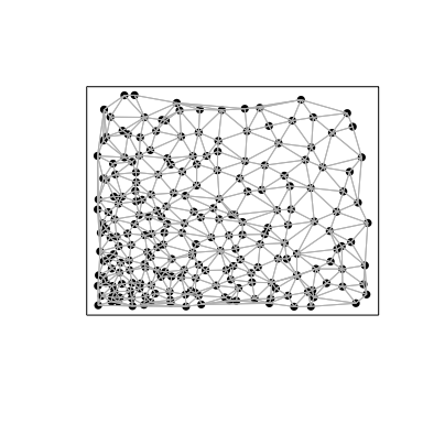
spatialCrossCor(gexp1, gexp2, weight)
par(mfrow=c(1,1), mar=rep(5,4))
spatialCrossCorTest(gexp1, gexp2, weight,
                    plot=TRUE)
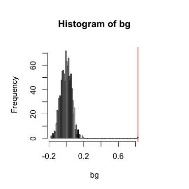
## [1] 0.8257857
## [1] 0.000999001
In this case, both the general and spatial cross-correlation statistics are positive.
Scenario 2: General cross-correlation and spatial cross-correlation suggest different trends
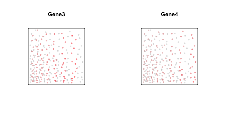
Now, let’s consider different two genes, Gene3 and Gene4. Gene3 is
expressed in a subset of cells along a gradient. Gene4 is expressed in
a different subset of cells, but along a similar gradient.
par(mfrow=c(1,2), mar=rep(5,4))
num <- pos[,1]

vi <- (num %% 2) == 0
gexp3 <- as.numeric(vi)
gexp3 <- gexp3 * sort(abs(rnorm(length(gexp3)))+1)
names(gexp3) <- rownames(pos)
plotEmbedding(posw, col=gexp3,
              main='Gene3')

vi <- (num %% 2) == 1
gexp4 <- as.numeric(vi)
gexp4 <- gexp4 * sort(abs(rnorm(length(gexp4)))+1)
names(gexp4) <- rownames(pos)
plotEmbedding(posw, col=gexp4,
              main='Gene4')
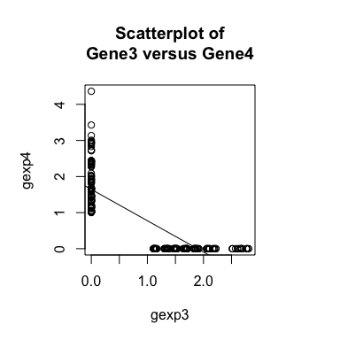
Now, if we plot the expression of Gene3 versus Gene4 in a
scatterplot, we see a negative relationship between the two genes are
expressed in different subsets of cells. Likewise, if we compute a
general cross-correlation statistic between Gene3 and Gene4, we can
identify a significant negative cross-correlation - that is, cells that
express higher levels of Gene3 tend to express lower levels of Gene4
and cells that express higher levels of Gene4 tend to express lower
levels of Gene3.
# Plot
par(mfrow=c(1,1), mar=rep(5,4))
plot(gexp3, gexp4,
     main='Scatterplot of\nGene3 versus Gene4')
abline(lm(gexp4~gexp3))
# Compute cross correlation
cor.test(gexp3, gexp4)

##
##  Pearson's product-moment correlation
##
## data:  gexp3 and gexp4
## t = -21.655, df = 223, p-value < 2.2e-16
## alternative hypothesis: true correlation is not equal to 0
## 95 percent confidence interval:
##  -0.8612940 -0.7760043
## sample estimates:
##        cor
## -0.8232408
However, if we compute a spatial cross-correlation statistic between
Gene3 and Gene4, we can identify a significant positive spatial
cross-correlation - that is, cells that express higher levels of Gene3
tend to be spatially neighboring cells that tend to express higher
levels of Gene4 and cells that express lower levels of Gene3 tend to
be spatially neighboring cells that tend to express lower levels of
Gene4.
# Compute spatial cross correlation
spatialCrossCor(gexp3, gexp4, weight)
par(mfrow=c(1,1), mar=rep(5,4))
spatialCrossCorTest(gexp3, gexp4, weight,
                    plot=TRUE)
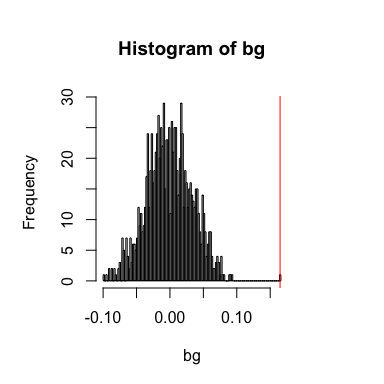
## [1] 0.1647783
## [1] 0.000999001
In this case, even though the general cross-correlation statistic is negative, the spatial cross-correlation statistic is positive.
This distinction is particularly important when we consider how
transcriptionally-distinct cell-types and subtypes may be interacting
with each other in space. For example, consider if Gene3 is a receptor
and Gene4 is a ligand. A general (spatially-unaware) cross-correlation
would not point us to any relationship between Gene3 and Gene4 other
than that they are expressed on different cell-types or subtypes. But a
spatial (spatially-aware) cross-correlation would hint at an
interaction.
Computing an inter-cell-type spatial cross-correlation
Now, let’s call cells that expression Gene3 cell-type A. And let’s
call cells that express Gene4 cell-type B. Note that cells of
cell-type A and cells of cell-type by are spatially intertwined.
ctA <- names(gexp3)[gexp3>0]
ctB <- names(gexp4)[gexp4>0]

# double check mutually exclusive
print(intersect(ctA, ctB))

# plot
par(mfrow=c(1,1), mar=rep(5,4))
cellType <- factor(rownames(posw) %in% ctA)
levels(cellType) <- c('ctB', 'ctA')
names(cellType) <- rownames(posw)
plotEmbedding(posw, groups=cellType,
              show.legend=TRUE,
              main='Cell Types in Space')
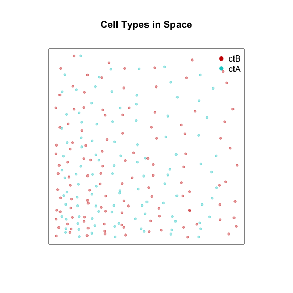
## character(0)
Now, instead of considering all neighbors, because we can see two
transcriptionally distinct but spatially intertwined cell-types in our
data, let’s only consider neighbor-relationships between cells of
cell-type A and cells of cell-type B. We can acheive this by modifying
the binary weight matrix used in the spatial cross-correlation statistic
calculation to include only neighbor-relationships between the two
cell-types (as opposed to within each cell-type). And indeed, we see a
very high inter-cell-type spatial cross-correlation - that is, cells of
cell-type A that express higher levels of Gene3 tend to be spatially
neighboring cells of cell-type B that tend to express higher levels of
Gene4 and cells of cell-type A that express lower levels of Gene3
tend to be spatially neighboring cells of cell-type B that tend to
express lower levels of Gene4, and vice versa.
par(mfrow=c(1,1), mar=rep(5,4))
weightIc <- getInterCellTypeWeight(ctA, ctB,
                                   weight, posw,
                                   plot=TRUE,
                                   main='Adjacency Weight Matrix\nBetween Cell-Types')
spatialCrossCor(gexp3, gexp4, weightIc)
interCellTypeSpatialCrossCor(gexp3, gexp4, ctA, ctB, weightIc)

spatialCrossCorTest(gexp3, gexp4, weightIc)

plotInterCellTypeSpatialCrossCor(gexp3, gexp4, ctA, ctB, weightIc,
                                 main='Spatial Cross Correlation')
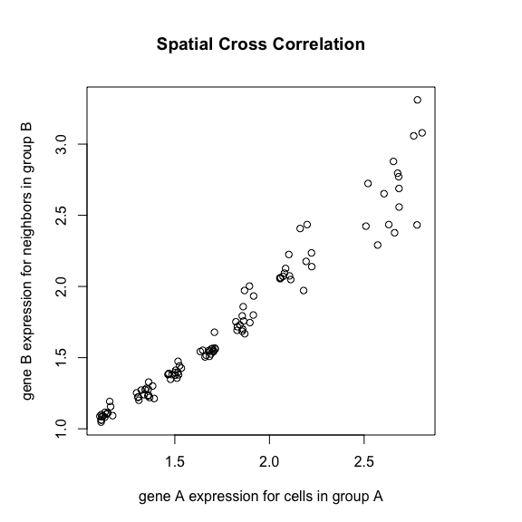
## [1] 0.9488357
## [1] -0.1200105
## [1] 0.000999001
Indeed, if Gene3 is a receptor and Gene4 is a ligand, the
observation that higher expression of the receptor in one cell-type is
always to spatially co-localized with higher expression of the ligand in
a different cell-type could be indicative of cellular interactions
between cell-Type A and B via these receptor-ligand complexes.
Scenario 3: Neither general cross-correlation nor spatial cross-correlation
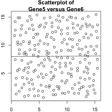
Lastly, let’s consider two genes, Gene5 and Gene6. Gene5 exhibits
a spatial gradient going from left to right. And Gene6 exhibits a
spatial gradient going from top to down.
par(mfrow=c(1,2), mar=rep(2,4))
set.seed(0)
gexp5 <- jitter(pos[,1], amount = 0.5)
names(gexp5) <- rownames(pos)
plotEmbedding(posw, col=gexp5,
              main='Gene5')

set.seed(1)
gexp6 <- jitter(pos[,2], amount = 0.5)
names(gexp6) <- rownames(pos)
plotEmbedding(posw, col=gexp6,
              main='Gene6')
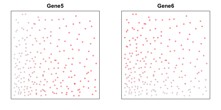
We observe no significant cross-correlation relationships between the two genes.
# Plot
par(mfrow=c(1,1), mar=rep(2,4))
plot(gexp5, gexp6, main='Scatterplot of\nGene5 versus Gene6')
abline(lm(gexp5~gexp6))
# Compute cross correlation
cor.test(gexp5, gexp6)

##
##  Pearson's product-moment correlation
##
## data:  gexp5 and gexp6
## t = 0.079181, df = 223, p-value = 0.937
## alternative hypothesis: true correlation is not equal to 0
## 95 percent confidence interval:
##  -0.1255754  0.1359986
## sample estimates:
##         cor
## 0.005302307
And also no significant spatial cross-correlation in this case.
# Compute spatial cross correlation
spatialCrossCor(gexp5, gexp6, weight)
par(mfrow=c(1,1), mar=rep(2,4))
spatialCrossCorTest(gexp5, gexp6, weight,
                    plot=TRUE)
## [1] 0.006021392
## [1] 0.9320679
Despite neither gene showing any spatial or general cross-correlation relationship between them, both genes can and do still exhibit high spatial auto-correlation in this example.
In summary, as these various simulated gene expression patterns highlight, spatial cross-correlation and autocorrelation can provide complementary information to general correlation analyses to enable the identification of potentially interesting spatial patterns indicative of cellular communication.