Reference-free cell-type deconvolution of multi-cellular spatially resolved transcriptomics data
Overview of STdeconvolve assumptions
STdeconvolve is built around latent Dirichlet allocation (LDA), which
seeks to represent latent “topics”, or cell-types, as ideally
non-overlapping groups of co-expressed, or frequently co-occurring,
genes in different pixels. In this manner, successful application of LDA
in deconvolving latent cell-types relies on several key assumptions that
can be reasonably met in ST data:
- It assumes that a few cell-types are present in each pixel. Given the micron-resolution pixel size in ST data and the average size of cells, we can generally assume that a single cell-type or a mixture of a few cell-types are present in each ST pixel
- We can assume that the proportional distribution of cell-types across pixels is heterogeneous within tissues profiled by ST such that some pixels will have more of one cell-type and other pixels will have more of another cell-type.
- As LDA represents latent cell-types as groups of co-expressed or
frequently co-occurring genes, it assumes that there will be
multiple genes informative of each underlying cell-type. While we
can generally assume this to be true for transcriptionally distinct
cell-types, this does mean that LDA, and subsequently
STdeconvolve, would not be suitable for resolving cell subtypes that are defined by very subtle combinations of minimally upregulated or downregulated genes with respect to other cell subtypes. - LDA, and subsequently
STdeconvolve, would not be able to differentiate between cell-types that cannot be distinguished through distinct differences in proportional gene expression such as volume or morphology. - LDA works best with a large number of documents. Consistent with this assumption, ST data measures the gene expression profiles of hundreds to thousands of spatially resolved pixels. Further, LDA works best when there are more documents than topics, else each document may be assigned to a different topic. For ST data, we can generally assume that there are more pixels than cell-types.
Selection of an appropriate model
Although STdeconvolve is a reference-free based deconvolution
approach, the number of cell-types, K, needs to be chosen a
priori. To determine the optimal number of cell-types K to choose for
a given dataset, we fit a set of LDA models using different values for
K over a user defined range of positive integers greater than 1.
For each LDA model, we compute it’s perplexity. The lower the
perplexity, the better the model represents the real dataset. Thus, the
trend between choice of K and the respective model perplexity can then
serve as a guide. STdeconvolve also reports the trend between K and
the number of deconvolved cell-types with mean pixel proportions < 5%
(as default). We chose this default threshold based on the difficulty of
STdeconvolve and reference-based deconvolution approaches to
deconvolve cell-types at low proportions, (i.e., “rare” cell-types). We
note that as K is increased for fitted LDA models, the number of such
“rare” cell-types generally increases. Such rare deconvolved cell-types
are often distinguished by fewer distinct transcriptional patterns in
the data and may represent non-relevant or spurious subdivisions of
primary cell-types. We can use this metric to help set an upper bound on
K.
Generally, perplexity decreases and the number of “rare” deconvolved cell-types increases as K increases. Given these model perplexities and number of “rare” deconvolved cell-types for each tested K, the optimal K can then be determined by choosing the maximum K with the lowest perplexity while minimizing number of “rare” deconvolved cell-types.
Still, for a given K, the fitted LDA model may fail to identify
distinct cell-types e.g., the distribution of cell-type proportions in
each pixel is uniform. In such a situation, the Dirichlet distribution
shape parameter α of the LDA model will be >= 1 and
STdeconvolve will indicate to the user that the fitted LDA model for a
particular K has an α above this threshold by graying out these Ks
in the trend plot.
Examples of different Dirichlet α’s
For an LDA model with a given K, the distribution of cell-type proportions for each pixel is drawn from a Dirichlet distribution with shape parameter α.
Assume we have a spatial transcriptomics dataset with 3 cell-types, (A, B, and C) and 100 pixels. The cell-type proportions of the pixels can be represented as 100 draws from the Dirichlet distribution, where a given draw is a 3-dimensional multinomial distribution, representing the probability of each cell-type in the pixel.
The cell-type probabilities of each multinomial distribution can be visualized on a probability simplex. In this case we have 3 dimensions so the simplex can be represented as a triangle and each multinomial distribution is a point on the triangle. The position of each point is dictated by it’s cell-type probabilities. For example, if we consider each multinomial probability distribution as a vector (A, B, C), then a point at the “A” corner of the simplex would be a multinomial probability distribution of (1, 0, 0), and have 100% probability of cell-type A and 0 for B and C. A point at the center of the simplex would have equal probability of each cell-type and it’s distribution would be (0.3, 0.3, 0.3).
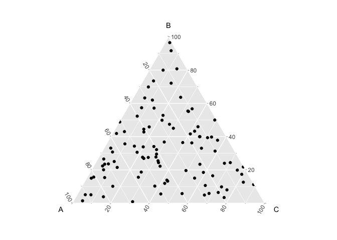
The Dirichlet distribution α controls the shape of the distribution of multinomials over the simplex. When α = 1, the Dirichlet distribution is uniform, which means that the multinomial distributions are drawn with equal chance across the simplex:
library(ggtern)
library(MCMCpack)
library(ggplot2)
set.seed(888)

alpha <- 1 ## Dirichlet shape parameter
pixels <- 100 ## i.e., number of draws
K <- 3 ## number of cell-types, i.e., number of dimensions

x <- MCMCpack::rdirichlet(pixels, rep(alpha, K))
colnames(x) <- LETTERS[1:K]
dat <- as.data.frame(x)
head(dat)
##           A          B         C
## 1 0.8190780 0.03810206 0.1428200
## 2 0.4621263 0.33841595 0.1994578
## 3 0.1977927 0.36243198 0.4397753
## 4 0.2738019 0.61970186 0.1064962
## 5 0.1389670 0.39962647 0.4614065
## 6 0.4382720 0.13209504 0.4296330
plt <- ggtern::ggtern(data = dat, ggplot2::aes(x = A, y = B, z = C))

plt + ggplot2::geom_point()
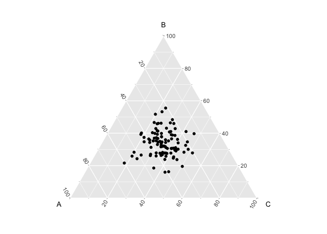
If α is > 1, then the multinomial distributions become centered in the simplex, which means that they tend to have equal probability of all three cell-types
set.seed(888)

alpha <- 10 ## Dirichlet shape parameter
pixels <- 100 ## i.e., number of draws
K <- 3 ## number of cell-types, i.e., number of dimensions

x <- MCMCpack::rdirichlet(pixels, rep(alpha, K))
colnames(x) <- LETTERS[1:K]
dat <- as.data.frame(x)
head(dat)
##           A         B         C
## 1 0.6018716 0.2158573 0.1822711
## 2 0.1741015 0.4102815 0.4156170
## 3 0.3489248 0.2775204 0.3735548
## 4 0.4025727 0.3427215 0.2547057
## 5 0.2057593 0.2783482 0.5158925
## 6 0.2881756 0.2905016 0.4213228
plt <- ggtern::ggtern(data = dat, ggplot2::aes(x = A, y = B, z = C))

plt + ggplot2::geom_point()
In this example, let’s visualize the probability of each cell-type for the first 10 pixels:
set.seed(888)

alpha <- 10 ## Dirichlet shape parameter
pixels <- 10 ## i.e., number of draws
K <- 3 ## number of cell-types, i.e., number of dimensions

x <- MCMCpack::rdirichlet(pixels, rep(alpha, K))

dat2 <- data.frame(item = factor(rep(1:K, pixels)),
                   draw = factor(rep(1:pixels, each = K)),
                   value = as.vector(t(x))
                   )

ggplot2::ggplot(data = dat2,
                ggplot2::aes(x=item, y=value, ymin=0, ymax=value)) +
                ggplot2::geom_point(colour=I("blue"))       +
                ggplot2::geom_linerange(colour=I("blue"))   +
                ggplot2::facet_wrap(~draw, ncol=5)          +
                ggplot2::scale_y_continuous(lim=c(0,1))     +
                ggplot2::theme(panel.border = ggplot2::element_rect(fill=0, colour="black")) +
                ggplot2::scale_x_discrete(labels=c("1" = "A", "2" = "B", "3" = "C")) +
                ggplot2::labs(x = "Cell-type", y = "probability", title = "Cell-type probability distribution of each pixel")
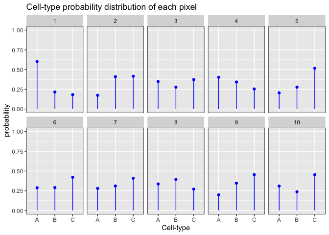
We can see that the cell-type probabilities are relatively the same within and between pixels.
If α < 1, then the multinomial distributions become concentrated towards the edges of the simplex.
set.seed(888)

alpha <- 0.1 ## Dirichlet shape parameter
pixels <- 100 ## i.e., number of draws
K <- 3 ## number of cell-types, i.e., number of dimensions

x <- MCMCpack::rdirichlet(pixels, rep(alpha, K))
colnames(x) <- LETTERS[1:K]
dat <- as.data.frame(x)
head(dat)
##              A            B            C
## 1 1.649651e-15 1.051135e-11 1.000000e+00
## 2 1.000000e+00 9.310912e-10 7.633010e-15
## 3 1.602978e-01 8.086178e-01 3.108447e-02
## 4 5.071938e-02 2.610649e-05 9.492545e-01
## 5 9.999947e-01 1.721919e-15 5.326931e-06
## 6 9.948597e-01 5.140343e-03 3.819135e-14
plt <- ggtern::ggtern(data = dat, ggplot2::aes(x = A, y = B, z = C))

plt + ggplot2::geom_point()
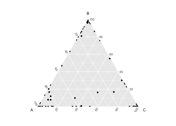
Now when we look at the probability distributions of the first 10 pixels, we see that each pixel is enriched for a given cell-type at different probabilities.
set.seed(888)

alpha <- 0.1 ## Dirichlet shape parameter
pixels <- 10 ## i.e., number of draws
K <- 3 ## number of cell-types, i.e., number of dimensions

x <- MCMCpack::rdirichlet(pixels, rep(alpha, K))

dat2 <- data.frame(item = factor(rep(1:K, pixels)),
                   draw = factor(rep(1:pixels, each = K)),
                   value = as.vector(t(x))
                   )

ggplot2::ggplot(data = dat2,
                ggplot2::aes(x=item, y=value, ymin=0, ymax=value)) +
                ggplot2::geom_point(colour=I("blue"))       +
                ggplot2::geom_linerange(colour=I("blue"))   +
                ggplot2::facet_wrap(~draw, ncol=5)          +
                ggplot2::scale_y_continuous(lim=c(0,1))     +
                ggplot2::theme(panel.border = ggplot2::element_rect(fill=0, colour="black")) +
                ggplot2::scale_x_discrete(labels=c("1" = "A", "2" = "B", "3" = "C")) +
                ggplot2::labs(x = "Cell-type", y = "probability", title = "Cell-type probability distribution of each pixel")
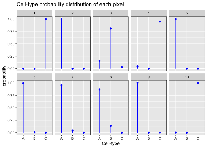
This fits with our assumption that the proportional distribution of cell-types across pixels is heterogeneous within tissues profiled by ST such that some pixels will have more of one cell-type and other pixels will have more of another cell-type.
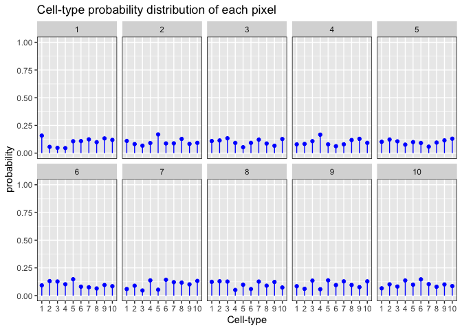
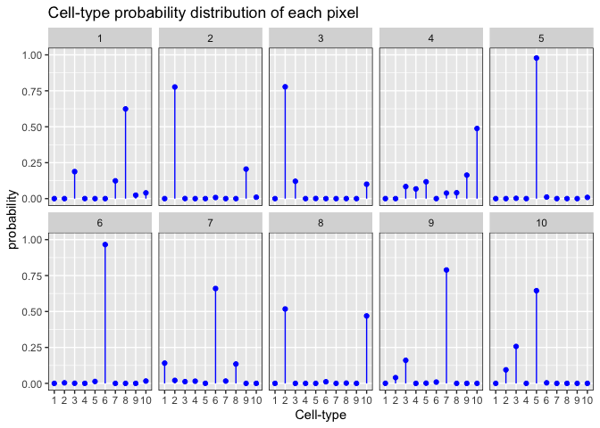
If we expand our example to a scenario in which we have 10 cell-types, we can see more clearly that when α > 1, each pixel is predicted to have an equal proportion of each cell-type, in which case the model is unable to deconvolve distinct cell-types in the pixels, compared to models where α < 1, and we are able to recover distinct cell-types in the pixels.
set.seed(888)

alpha <- 10 ## Dirichlet shape parameter
pixels <- 10 ## i.e., number of draws
K <- 10 ## number of cell-types, i.e., number of dimensions

x <- MCMCpack::rdirichlet(pixels, rep(alpha, K))

dat2 <- data.frame(item = factor(rep(1:K, pixels)),
                   draw = factor(rep(1:pixels, each = K)),
                   value = as.vector(t(x))
                   )

ggplot2::ggplot(data = dat2,
                ggplot2::aes(x=item, y=value, ymin=0, ymax=value)) +
                ggplot2::geom_point(colour=I("blue"))       +
                ggplot2::geom_linerange(colour=I("blue"))   +
                ggplot2::facet_wrap(~draw, ncol=5)          +
                ggplot2::scale_y_continuous(lim=c(0,1))     +
                ggplot2::theme(panel.border = ggplot2::element_rect(fill=0, colour="black")) +
                ggplot2::labs(x = "Cell-type", y = "probability", title = "Cell-type probability distribution of each pixel")
set.seed(888)

alpha <- 0.1 ## Dirichlet shape parameter
pixels <- 10 ## i.e., number of draws
K <- 10 ## number of cell-types, i.e., number of dimensions

x <- MCMCpack::rdirichlet(pixels, rep(alpha, K))

dat2 <- data.frame(item = factor(rep(1:K, pixels)),
                   draw = factor(rep(1:pixels, each = K)),
                   value = as.vector(t(x))
                   )

ggplot2::ggplot(data = dat2,
                ggplot2::aes(x=item, y=value, ymin=0, ymax=value)) +
                ggplot2::geom_point(colour=I("blue"))       +
                ggplot2::geom_linerange(colour=I("blue"))   +
                ggplot2::facet_wrap(~draw, ncol=5)          +
                ggplot2::scale_y_continuous(lim=c(0,1))     +
                ggplot2::theme(panel.border = ggplot2::element_rect(fill=0, colour="black")) +
                ggplot2::labs(x = "Cell-type", y = "probability", title = "Cell-type probability distribution of each pixel")
Therefore, when choosing an optimal model for a given K, we also want
models in which α < 1. When fitting LDA models, STdeconvolve
not only tracks the perplexity and % of rare cell-types, but will also
indicate to users models in which α > 1 by shading them out on
the plot returned by fitLDA().
STdeconvolve failures
model where α > 1
To illustrate the above point, let’s fit several LDA models to the mOB
test data that result in some models with an α > 1.
An α > 1 is indicates that the LDA was not able to deconvolve distinct cell-types in the pixels. The most likely reason for this is that the selected features (genes) included in the input dataset were not sufficient to distinguish between transcirptionally distinct cell-types.
To illustrate this point, let’s create an input dataset just using randomly sampled genes. Here, we are not selecting for overdispersed genes as a means to detect cell-type specific transcriptional profiles. We do not expect the random genes to provide enough information for the model to identify latent cell-types (i.e., non-overlapping groups of co-expressed, or frequently co-occurring, genes) in different pixels.
library(STdeconvolve)
data(mOB)
pos <- mOB$pos
cd <- mOB$counts
annot <- mOB$annot
set.seed(888)

## filter genes
counts <- cleanCounts(counts = cd,
                      min.lib.size = 100,
                      min.reads = 1,
                      min.detected = 1,
                      plot = FALSE)

## random genes
genes <- sample(x = rownames(as.matrix(counts)), size = 100)

## build corpus using just the selected genes
mobCorpus2 <- preprocess(t(cd),
                       selected.genes = genes,
                       # can then proceed to filter this list, if desired
                       # min.reads = 1,
                       min.lib.size = 1, # can still filter pixels
                       min.detected = 1, # can still filter to make sure the selected genes are present in at least 1 pixel
                       ODgenes = FALSE, # don't select the over dispersed genes
                       verbose = FALSE)
## Final corpus:

## A 260x100 simple triplet matrix.

## Preprocess complete.
## fit LDA models to the corpus
ks <- seq(from = 2, to = 12, by = 1) # range of K's to fit LDA models with given the input corpus
ldas <- fitLDA(as.matrix(mobCorpus2$corpus),
               Ks = ks,
               ncores = parallel::detectCores(logical = TRUE) - 1, # number of cores to fit LDA models in parallel
               plot=TRUE, verbose=TRUE)
## Warning in serialize(data, node$con): 'package:stats' may not be available
## when loading

## Warning in serialize(data, node$con): 'package:stats' may not be available
## when loading

## Warning in serialize(data, node$con): 'package:stats' may not be available
## when loading

## Warning in serialize(data, node$con): 'package:stats' may not be available
## when loading

## Warning in serialize(data, node$con): 'package:stats' may not be available
## when loading

## Warning in serialize(data, node$con): 'package:stats' may not be available
## when loading

## Warning in serialize(data, node$con): 'package:stats' may not be available
## when loading

## Time to fit LDA models was 0.11 mins

## Computing perplexity for each fitted model...

## Warning in serialize(data, node$con): 'package:stats' may not be available
## when loading

## Warning in serialize(data, node$con): 'package:stats' may not be available
## when loading

## Warning in serialize(data, node$con): 'package:stats' may not be available
## when loading

## Warning in serialize(data, node$con): 'package:stats' may not be available
## when loading

## Warning in serialize(data, node$con): 'package:stats' may not be available
## when loading

## Warning in serialize(data, node$con): 'package:stats' may not be available
## when loading

## Warning in serialize(data, node$con): 'package:stats' may not be available
## when loading

## Time to compute perplexities was 0.17 mins

## Getting predicted cell-types at low proportions...

## Time to compute cell-types at low proportions was 0 mins

## Plotting...
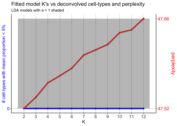
Here, the LDA models have α’s > 1.
We can obtain the α’s for each model via:
unlist(sapply(ldas$models, slot, "alpha"))
##         2         3         4         5         6         7         8
##  80.18376 141.21467 137.74855 141.81926 137.81350 124.85134 122.69297
##         9        10        11        12
## 119.42429 109.37748 108.52553 100.51034
Let’s check out the results for K = 12.
optLDA <- optimalModel(models = ldas, opt = 12)
results <- getBetaTheta(optLDA, perc.filt = 0.05, betaScale = 1000)
## Filtering out cell-types in pixels that contribute less than 0.05 of the pixel proportion.
deconProp <- results$theta
deconGexp <- results$beta
vizAllTopics(deconProp, pos, r=0.4, lwd = 0.1)
## Plotting scatterpies for 260 pixels with 12 cell-types...this could take a while if the dataset is large.
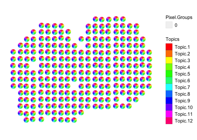
As expected, using only random genes did not provide enough information
for the model to identify latent cell-types (i.e., non-overlapping
groups of co-expressed, or frequently co-occurring, genes) in the
pixels. As a result, the α’s are very large for all of the fitted
LDA models. STdeconvolve indicates this by shading the models for
which α > 1. Again, note that the cell-type distributions are
uniform in the pixels.
Instead, let’s try fitting LDA models using feature selected overdispersed genes to serve as a proxy for identifying cell-type transcriptional profiles. We will limit the overdispersed genes to the top 100 to be consistent with the number of randomly selected genes.
counts <- cleanCounts(counts = cd,
                      min.lib.size = 100,
                      min.reads = 1,
                      min.detected = 1,
                      plot = FALSE)

odGenes <- getOverdispersedGenes(as.matrix(counts),
                      gam.k=5,
                      alpha=0.05,
                      plot=FALSE,
                      use.unadjusted.pvals=FALSE,
                      do.par=TRUE,
                      max.adjusted.variance=1e3,
                      min.adjusted.variance=1e-3,
                      verbose=FALSE, details=FALSE)

# limit the number of overdispersed genes when building the input corpus
genes <- odGenes[1:100]

## build corpus using just the selected genes
mobCorpus2 <- preprocess(t(cd),
                       selected.genes = genes,
                       # can then proceed to filter this list, if desired
                       # min.reads = 1,
                       min.lib.size = 1, # can still filter pixels
                       min.detected = 1, # can still filter to make sure the selected genes are present in at least 1 pixel
                       ODgenes = FALSE, # don't select the over dispersed genes
                       verbose = FALSE)
## Final corpus:

## A 260x100 simple triplet matrix.

## Preprocess complete.
## fit LDA models to the corpus
ks <- seq(from = 2, to = 12, by = 1) # range of K's to fit LDA models with given the input corpus
ldas <- fitLDA(as.matrix(mobCorpus2$corpus),
               Ks = ks,
               ncores = parallel::detectCores(logical = TRUE) - 1, # number of cores to fit LDA models in parallel
               plot=TRUE, verbose=TRUE)
## Warning in serialize(data, node$con): 'package:stats' may not be available
## when loading

## Warning in serialize(data, node$con): 'package:stats' may not be available
## when loading

## Warning in serialize(data, node$con): 'package:stats' may not be available
## when loading

## Warning in serialize(data, node$con): 'package:stats' may not be available
## when loading

## Warning in serialize(data, node$con): 'package:stats' may not be available
## when loading

## Warning in serialize(data, node$con): 'package:stats' may not be available
## when loading

## Warning in serialize(data, node$con): 'package:stats' may not be available
## when loading

## Time to fit LDA models was 0.4 mins

## Computing perplexity for each fitted model...

## Warning in serialize(data, node$con): 'package:stats' may not be available
## when loading

## Warning in serialize(data, node$con): 'package:stats' may not be available
## when loading

## Warning in serialize(data, node$con): 'package:stats' may not be available
## when loading

## Warning in serialize(data, node$con): 'package:stats' may not be available
## when loading

## Warning in serialize(data, node$con): 'package:stats' may not be available
## when loading

## Warning in serialize(data, node$con): 'package:stats' may not be available
## when loading

## Warning in serialize(data, node$con): 'package:stats' may not be available
## when loading

## Time to compute perplexities was 0.16 mins

## Getting predicted cell-types at low proportions...

## Time to compute cell-types at low proportions was 0 mins

## Plotting...
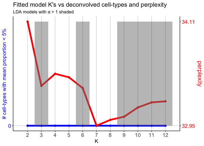
unlist(sapply(ldas$models, slot, "alpha"))
##         2         3         4         5         6         7         8
## 0.9233002 1.0155469 0.9646652 0.9967726 1.0883712 0.9445329 0.9750063
##         9        10        11        12
## 1.0340109 1.0559614 1.1231159 1.1946524
Here, let’s choose the model K = 7, because it has the lowest perplexity, number of rare cell-types is 0, and the α < 1.
optLDA <- optimalModel(models = ldas, opt = 7)
results <- getBetaTheta(optLDA, perc.filt = 0.05, betaScale = 1000)
## Filtering out cell-types in pixels that contribute less than 0.05 of the pixel proportion.
deconProp <- results$theta
deconGexp <- results$beta
vizAllTopics(deconProp, pos, r=0.4, lwd = 0.1)
## Plotting scatterpies for 260 pixels with 7 cell-types...this could take a while if the dataset is large.
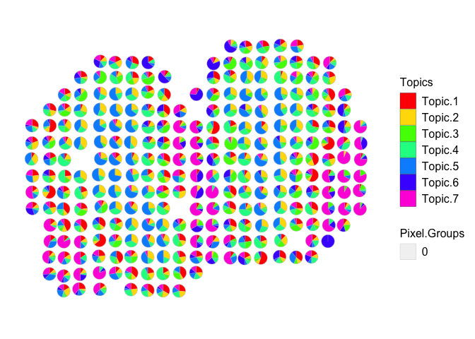
Now we are able to see distinct cell-types across the pixels. Importantly, most pixels are enriched for just a few cell-types, as we would expect.