Reference-free cell-type deconvolution of multi-cellular spatially resolved transcriptomics data
The following code demonstrates how to create the DBiT-seq input matrix
for STdeconvolve, which was used for analyses in the STdeconvolve
paper.
This was based on the GSM4364242 dataset of a mouse E11 lower embryo and tail section.
library(STdeconvolve)
Process raw data
dbit_e11_counts <- read.csv("./GSE137986_RAW/GSM4364242_E11-1L.tsv",
                            sep = "\t",
                            row.names = 1)

## 20849 genes by 1837 pixels
dbit_e11_counts <- as(t(dbit_e11_counts), "dgCMatrix")
dbit_e11_counts
## 20849 x 1837 sparse Matrix of class "dgCMatrix"

##    [[ suppressing 29 column names '10x35', '10x34', '10x33' ... ]]
##    [[ suppressing 29 column names '10x35', '10x34', '10x33' ... ]]

##
## Rp1     . . . . . . . . . . . . . . . . . . . . . . . . . . . . . ......
## Sox17   . . . . . . . . . . . . . . 1 . . . . . . . . . . . . . . ......
## Gm37587 . . . . . . . . . . . . . . . . . . . . . . . . . . . . . ......
## Gm7357  . . . . . . . . . . . . . . . . . . . . . . . . . . . . . ......
## Gm7369  . . . . . . . . . . . . . . . . . . . . . . . . . . . . . ......
## Gm6085  . . . 2 . 3 1 2 . . 3 3 . . . . . . . 2 . . . 1 . . . . . ......
## Gm6123  . . . . . . . . . . . . . . . . . . . . . . . . . . . . . ......
## Gm37144 . . . . . . . . . . . . . . . . . . . . . . . . . . . . . ......
## Mrpl15  . 1 . . . . . . . . . . . . . 1 . . 1 . . 1 . . . 1 . . . ......
## Lypla1  . . . . . . . . . . . . . . . . . 1 . . . . . . . . . . . ......
## Gm6104  . . . . . . . . . . . . . . . . . . . . . . . . . . . . . ......
## Tcea1   . 1 . . . 2 1 1 . 1 . 1 1 . . . . . . . . . . . . . . . . ......
## Gm17100 . . . . . . . . . . . . . . . . . . . . . . . . . . . . . ......
## Rgs20   . . . . . . . . . . . . . . . . . . . . . . . . . . . . . ......
## Atp6v1h . . . . . . . . . . . . . . . . . . . . . 1 1 . . . . . . ......
## Oprk1   . . . . . . . . . . . . . . . . . . . . . . . . . . . . . ......
## Npbwr1  . . . . . . . . . . . . . . . . . . . . . . . . . . . . . ......
##
##  ..............................
##  ........suppressing 1808 columns and 20815 rows in show(); maybe adjust 'options(max.print= *, width = *)'
##  ..............................

##    [[ suppressing 29 column names '10x35', '10x34', '10x33' ... ]]

##
## mt.Tc   . . . .  .  . . . .  . . . . . . . . . . . . . . . . . . . . ......
## mt.Ty   . . . .  .  . . . .  . . . . . . . . . . . . . . . . . . . . ......
## mt.Co1  6 6 3 9 13 14 7 7 4  8 6 1 8 3 7 3 1 4 2 1 6 5 7 . . . 1 . 2 ......
## mt.Ts1  . . . .  .  . . . .  . . . . . . . . . . . . . . . . . . . . ......
## mt.Td   . . . .  .  . . . .  . . . . . . . . . . . . . . . . . . . . ......
## mt.Co2  3 2 2 2  3  4 4 1 2  6 1 2 1 2 1 1 . . . 1 3 . 1 . . . . . . ......
## mt.Atp8 . . . .  .  . . . .  . . . . . . . . . . . . . . . . . . . . ......
## mt.Atp6 . 2 . 2  1  3 1 3 .  1 . . 2 2 1 . . 3 1 1 1 1 . . . . . . . ......
## mt.Co3  4 7 5 9  5 15 7 5 6 10 8 7 7 2 5 5 2 2 7 2 . 4 3 . . . . 2 . ......
## mt.Nd3  . . . .  1  1 . . 2  . . . . . . . . 1 . . . . . . . . . . . ......
## mt.Nd4l . . . .  .  . . . .  . . . . . . 1 . . . . . . . . . . . . . ......
## mt.Nd4  3 . 1 1  1  2 . 2 2  1 1 . 1 . 1 . 1 . 1 3 2 3 . . . . . . . ......
## mt.Nd5  . . 1 .  2  . 2 1 1  . 2 . . . . . . . 2 1 . 1 2 . . . . . . ......
## mt.Nd6  . . . .  .  . . . .  . . . . . . . . . . . . . . . . . . . . ......
## mt.Cytb 1 1 2 5  5  4 4 5 5  1 3 1 2 2 4 2 1 2 3 1 3 3 1 . . . . . 2 ......
## mt.Tt   . . . .  .  . . . .  . . . . . . . . . . . . . . . . . . . . ......
## mt.Tp   . . . .  .  . . . .  . . . . . . . . . . . . . . . . . . . . ......
Note that the pixel IDs are essentially named based on their x-y coordinates.
## remove mt genes:
dbit_e11_counts <- dbit_e11_counts[!grepl("mt.", rownames(dbit_e11_counts)), ]
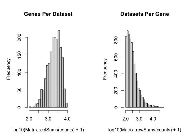
dbit_e11_clean <- cleanCounts(dbit_e11_counts,
min.lib.size = 100,
max.lib.size = Inf,
min.reads = 100,
min.detected = 1,
verbose = TRUE,
plot=TRUE)
## Filtering matrix with 1837 cells and 20707 genes ...

## Resulting matrix has 1832 cells and 7171 genes
dbit_e11_corpus <- preprocess(t(as.matrix(dbit_e11_clean)),
alignFile = NA,
extractPos = TRUE, ## extract the x-y coodiantes from the pixel IDs
selected.genes = NA,
nTopGenes = NA,
genes.to.remove = NA,
removeAbove = 0.95, ## remove genes in more than 95% pixels
removeBelow = 0.05, ## remove genes in less than 5% of pixels
min.lib.size = 100, ## keep pixels with 100+ gene counts
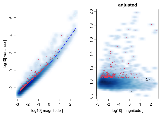
ODgenes = TRUE,
nTopOD = 1000, ## limit to top 1000 overdispersed genes
od.genes.alpha = 0.01, ## only overdispersed genes with p.adj < 0.01
gam.k = 5,
verbose = TRUE)
## Initial genes: 7171 Initial pixels: 1832

## - Removing poor pixels with <= 100 reads

## - Removing genes with <= 1 reads across pixels and detected in <= 1 pixels

##   Remaining genes: 7171 and remaining pixels: 1831

## - Removed genes present in 95% or more of pixels
##  Remaining genes: 7157

## - Removed genes present in 5% or less of pixels
##  Remaining genes: 6829

## - Capturing only the overdispersed genes...

## Converting to sparse matrix ...

## Calculating variance fit ...

## Using gam with k=5...

## 1023 overdispersed genes ...

## - Using top 1000 overdispersed genes.

## - Check that each pixel has at least 1 non-zero gene count entry..

## Final corpus:

## A 1831x1000 simple triplet matrix.

## Extracting positions from pixel names.

## Preprocess complete.
The y-axis needs to be reversed.
dbit_e11_corpus$posR <- dbit_e11_corpus$pos
dbit_e11_corpus$posR[, "y"] <- dbit_e11_corpus$posR[, "y"] * -1
Make gene count dataframe with positions to use with vizGeneCounts
geneDf_e11 <- merge(as.data.frame(dbit_e11_corpus$posR),
            as.data.frame(as.matrix(dbit_e11_corpus$corpus)),
            by = 0)
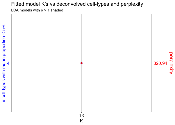
LDA model fitting
## for E11, in paper there were 13 clusters.
ks <- c(13)

dbit_e11_LDAs <- fitLDA(counts = as.matrix(dbit_e11_corpus$corpus),
                        Ks = ks,
                        perc.rare.thresh = 0.05,
                        seed = 0,
                        ncores = 7,
                        plot = TRUE)
## Warning in serialize(data, node$con): 'package:stats' may not be available
## when loading

## Time to fit LDA models was 3.94 mins

## Computing perplexity for each fitted model...

## Warning in serialize(data, node$con): 'package:stats' may not be available
## when loading

## Time to compute perplexities was 0.07 mins

## Getting predicted cell-types at low proportions...

## Time to compute cell-types at low proportions was 0 mins

## Plotting...

## geom_path: Each group consists of only one observation. Do you need to
## adjust the group aesthetic?
## geom_path: Each group consists of only one observation. Do you need to
## adjust the group aesthetic?
Check the alphas of the fitted models
unlist(sapply(dbit_e11_LDAs$models, slot, "alpha"))
##        13
## 0.1021903
Deconvolve the cell-types for each fitted model. Store in a list to access
optLDA <- optimalModel(models = dbit_e11_LDAs, opt = 13)
results <- getBetaTheta(lda = optLDA,
                        perc.filt = 0.05, # remove cell-types from pixels that are predicted to be present at less than 5%. Then readjust pixel proportions to 100%
                        betaScale = 1000) # scale the cell-type transcriptional profiles
## Filtering out cell-types in pixels that contribute less than 0.05 of the pixel proportion.
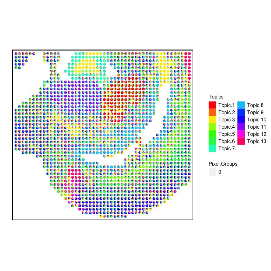
Visualize K=13
m <- results$theta
pos <- dbit_e11_corpus$posR

p <- vizAllTopics(theta = m,
                   pos = pos,
                   topicOrder = seq(ncol(m)),
                   r = 0.4,
                   lwd = 0,
                   showLegend = TRUE,
                   plotTitle = NA) +
  ggplot2::guides(fill=ggplot2::guide_legend(ncol=2)) +

  ## outer border
  ggplot2::geom_rect(data = data.frame(pos),
            ggplot2::aes(xmin = min(x)-1, xmax = max(x)+1,
                         ymin = min(y)-1, ymax = max(y)+1),
            fill = NA, color = "black", linetype = "solid", size = 0.5) +

  ggplot2::theme(
    plot.background = ggplot2::element_blank()
  ) +

  ggplot2::coord_equal()
## Plotting scatterpies for 1831 pixels with 13 cell-types...this could take a while if the dataset is large.

## Coordinate system already present. Adding new coordinate system, which will replace the existing one.
p