Clusters of Genes Expressing ERBB2 using t-SNE

What data types are you visualizing?
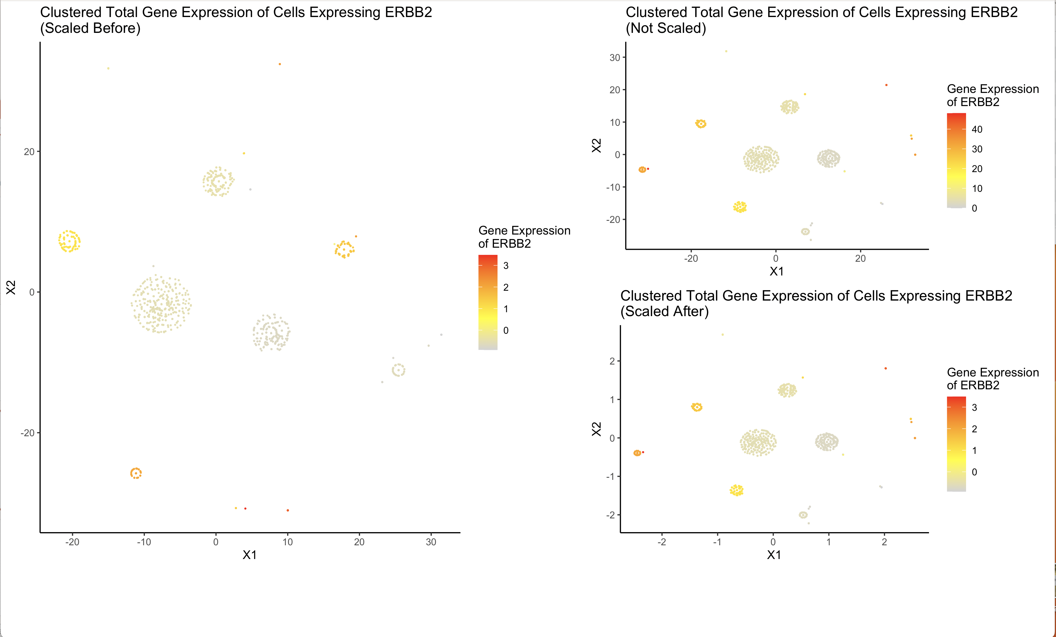
I am visualizing the similarities in levels of overall gene expression in cells that have non-zero expression of ERBB2 and the level of expression of ERBB2 as well as the difference between scaling data before and after dimensionality reduction.
What data encodings are you using to visualize these data types?
I am using the geometric primitive of points to represent each cell. I am using the visual channel of hue to represent levels of gene expression of ERBB2.
What type of data visualization is this? What about the data are you trying to make salient through this data visualization?
My data visualization attempts to use dimension reduction to make more salient the relationship between cell type and level of ERBB2 visualization. ERBB2 is the most widely expressed gene in the data, by doing dimensionality reduction (t-SNE) on cells that have a non-zero expression of ERBB2, clusters of cells appear which indicate similarity across all genes expressed. Each of these clusters also has a similar hue which indicates that the similarities are also related to the total expression of ERBB2 in each cell. Futher, I am also trying to visualize the difference between using the scale() function before and after Rtsne(). The greatest impact seems to be on outliers between the two cases. Scaling after pretty obviously reflects no scaling on the data. The optimal choice seems to be scaling before as it has a more desirable impact on grouping outliers.
What Gestalt principles or knowledge about perceptiveness of visual encodings are you using to accomplish this?
I am using the Gestalt principles of proximity and similarity (i.e. chart size) to emphasize the two groups of charts, the optimal data visualization (scale before) which is larger in height and width and the comparison (no scaling or scaling after) which are smaller and of equal size indicating similarity.
Code
data <- read.csv(‘bulbasaur.csv.gz’) dim(data) head(data)
#initialization attribution: Prof. Fan in class
gexp <- data[,5:ncol(data)]
#find max expressed gene totgenes <- colSums(gexp) max_expression = which(totgenes == max(totgenes))
ERBB2.cells<- gexp[“ERBB2”> 0] mat <- gexp[ERBB2.cells[,1],] mat.scale <- scale(mat)
source: https://www.statology.org/remove-columns-with-na-in-r/
mat.scale <- mat.scale[ , colSums(is.na(mat.scale))==0]
#tSNE
#variable assigning, dataframe creation, and ggplot inspiration attribution: Prof. Fan in class library(Rtsne) emb1 <- Rtsne(mat,check_duplicates = FALSE) emb2 <- Rtsne(mat.scale,check_duplicates = FALSE)
library(ggplot2) df1 <- data.frame(emb1$Y, relative_gene_expression = mat[,”ERBB2”]) df2 <- data.frame(emb2$Y, relative_gene_expression = mat.scale[,”ERBB2”]) df3 <- data.frame(scale(emb1$Y), relative_gene_expression = scale(mat[,”ERBB2”]))
p1 <- ggplot(df1,aes(x=X1,y=X2,col = relative_gene_expression)) + geom_point(size = 0.2) + scale_color_gradientn(colors = c(“lightgrey”, “yellow”, “orange”, “red”)) + ggtitle(“Clustered Total Gene Expression of Cells Expressing ERBB2 \n(Not Scaled)”) + theme_classic() + labs(color = “Gene Expression \nof ERBB2”)
p2 <- ggplot(df2,aes(x=X1,y=X2,col = relative_gene_expression)) + geom_point(size = 0.2) + scale_color_gradientn(colors = c(“lightgrey”, “yellow”, “orange”, “red”)) + ggtitle(“Clustered Total Gene Expression of Cells Expressing ERBB2 \n(Scaled Before)”) + theme_classic() + labs(color = “Gene Expression \nof ERBB2”)
p3 <- ggplot(df3,aes(x=X1,y=X2,col = relative_gene_expression)) + geom_point(size = 0.2) + scale_color_gradientn(colors = c(“lightgrey”, “yellow”, “orange”, “red”)) + ggtitle(“Clustered Total Gene Expression of Cells Expressing ERBB2 \n(Scaled After)”) + theme_classic() + labs(color = “Gene Expression \nof ERBB2”)
source: https://stackoverflow.com/questions/36198451/specify-widths-and-heights-of-plots-with-grid-arrange
library(gridExtra) grid.arrange(arrangeGrob(p2, ncol=1, nrow=1), arrangeGrob(p1,p3, ncol=1, nrow=2), heights=c(4,.5), widths=c(1.25,1))