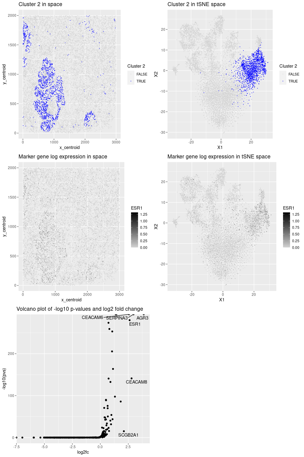
Differentially expressed genes and cell-type annotation for cluster 2

Cell-type annotation
For this data visualization, we selected cluster 2 as it presented an interesting pattern. Then, by performing kmeans clustering and differential analysis on the normalized data, we noticed that it has some breast cancer markers such as ERBB2, ESR1, GATA3, and AGR3 (as confirmed in the protein atlas https://www.proteinatlas.org/). In addition, some of those genes (ESR1, AGR3) had the highest fold change and p-values, indicating their importance to represent the cluster. Therefore, cluster 2 corresponds to a breast cancer cell type.
Please share the code you used to reproduce this data visualization.
library(tidyverse)
library(gridExtra)
library(ggrepel)
set.seed(42)

# Preprocessing -----------------------------------------------------------

## load data
data <- read.csv("./data/pikachu.csv.gz", row.names = 1)
dim(data)
pos <- data[, 1:2]
area <- data[, 3]
gexp <- data[4:ncol(data)]

## remove empty cells
good_cells <- rownames(gexp)[rowSums(gexp) > 0]
pos <- pos[good_cells, ]
area <- area[good_cells]
gexp <- gexp[good_cells, ]

## normalize
totgexp <- rowSums(gexp)
mat <- gexp/totgexp
mat <- mat*100
mat <- log10(mat + 1)


# Reduced dimension and clustering ----------------------------------------

## calculate tsne
emb <- Rtsne::Rtsne(mat, check = F)

## calculate multiple k means and select k value
kmeans_ss <- lapply(1:15, FUN = function(x){
    com <- kmeans(mat, centers = x)
    kmeans_vals <- list(wss = com$tot.withinss,
                        bss = com$betweenss,
                        clusters = com$cluster)
    return(kmeans_vals)
})

df_ss <- data.frame(k = 1:15,
                    wss = sapply(kmeans_ss, "[[", 1),
                    bss = sapply(kmeans_ss, "[[", 2))

p_wss <- df_ss %>% ggplot() +
    geom_line(aes(x=k, y=wss))
p_bss <- df_ss %>% ggplot() +
    geom_line(aes(x=k, y=bss))

grid.arrange(p_wss, p_bss)

## based on the graphs, I chose k = 8
com <- kmeans(mat, centers = 8)
clusters <- com$cluster

## colorblind-friendly palette: http://www.cookbook-r.com/Graphs/Colors_(ggplot2)/
cbbPalette <- c("#000000", "#E69F00", "#56B4E9", "#009E73", "#F0E442", "#0072B2", "#D55E00", "#CC79A7")

## visualize clusters
pos %>%
    mutate(cluster = as.factor(clusters)) %>%
    ggplot() +
    geom_point(aes(x_centroid, y_centroid, color = cluster),
               size = .5) +
    scale_color_manual(values = cbbPalette) +
    guides(colour = guide_legend(override.aes = list(size=5)))

## cluster 2 has a nice spatial pattern
plot_clus_pos <- pos %>%
    mutate(cluster = as.factor(clusters)) %>%
    ggplot() +
    geom_point(aes(x_centroid, y_centroid, color = cluster == 2),
               size = .1) +
    scale_color_manual(values = c("lightgray", "blue")) +
    labs(title = "Cluster 2 in space", color = "Cluster 2")


plot_clus_emb <- emb$Y %>%
    data.frame() %>%
    mutate(cluster = as.factor(clusters)) %>%
    ggplot() +
    geom_point(aes(X1, X2, color = cluster == 2),
               size = .1) +
    scale_color_manual(values = c("lightgray", "blue")) +
    labs(title = "Cluster 2 in tSNE space", color = "Cluster 2")


# Differentially expressed genes ------------------------------------------

## select a cluster
selected_cluster <- 2
cluster_of_interest <- names(which(clusters == selected_cluster))
other_clusters <- names(which(clusters != selected_cluster))

## loop through the genes and test each one
genes <- colnames(mat)
pvs <- sapply(genes, function(g){
    a <- mat[cluster_of_interest, g]
    b <- mat[other_clusters, g]
    wilcox.test(a, b, alternative = "greater")$p.val
})

## see marker genes
names(which(pvs < 1e-8))

## "ERBB2" and "ESR1" are breast cancer marker genes
## https://www.proteinatlas.org/ENSG00000141736-ERBB2
## https://www.proteinatlas.org/ENSG00000091831-ESR1
pos %>%
    mutate(gene = mat$ESR1) %>%
    ggplot() +
    geom_point(aes(x_centroid, y_centroid, color = gene),
               size = .1) +
    scale_color_gradient(low = "lightgray", high = "black")

emb$Y %>%
    data.frame() %>%
    mutate(gene = mat$ESR1) %>%
    ggplot() +
    geom_point(aes(X1, X2, color = gene),
               size = .1) +
    scale_color_gradient(low = "lightgray", high = "black")

head(sort(pvs))
g <- names(sort(pvs))[1]
g
## AGR3: Breast cancer marker
## https://www.proteinatlas.org/ENSG00000173467-AGR3
pos %>%
    mutate(gene = mat[,g]) %>%
    ggplot() +
    geom_point(aes(x_centroid, y_centroid, color = gene),
               size = .1) +
    scale_color_gradient(low = "lightgray", high = "black") +
    labs(title = "Marker gene expression in space", color = g)


emb$Y %>%
    data.frame() %>%
    mutate(gene = mat[,g]) %>%
    ggplot() +
    geom_point(aes(X1, X2, color = gene),
               size = .1) +
    scale_color_gradient(low = "lightgray", high = "black") +
    labs(title = "Marker gene expression in tSNE space", color = g)

## for ESR1
g <- "ESR1"
plot_gene_pos <- pos %>%
    mutate(gene = mat[,g]) %>%
    ggplot() +
    geom_point(aes(x_centroid, y_centroid, color = gene),
               size = .1) +
    scale_color_gradient(low = "lightgray", high = "black") +
    labs(title = "Marker gene log expression in space", color = g)


plot_gene_emb <- emb$Y %>%
    data.frame() %>%
    mutate(gene = mat[,g]) %>%
    ggplot() +
    geom_point(aes(X1, X2, color = gene),
               size = .1) +
    scale_color_gradient(low = "lightgray", high = "black") +
    labs(title = "Marker gene log expression in tSNE space", color = g)

## calculate a fold change
log2fc <- sapply(genes, function(g){
    a <- mat[cluster_of_interest, g]
    b <- mat[other_clusters, g]
    log2(mean(a)/mean(b))
})

pvs[g]
log2fc[g]

tail(sort(log2fc))

## half volcano plot
df <- data.frame(pvs, log2fc)
head(df)
plot_deg <- df %>%
    ggplot(aes(log2fc, -log10(pvs))) +
    geom_point() +
    geom_text_repel(aes(label = ifelse(log2fc > 2.1, as.character(rownames(df)), '')),
              hjust=0, vjust=0) +
    labs(title = "Volcano plot of -log10 p-values and log2 fold change")

## join all plots
grid.arrange(plot_clus_pos, plot_clus_emb,
            plot_gene_pos, plot_gene_emb,
            plot_deg)