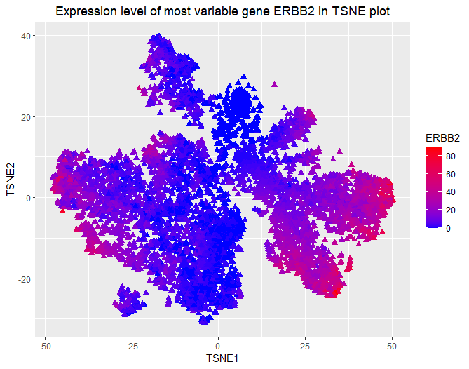
Expression level of the most variable gene ERBB2 in TSNE plot

What data types are you visualizing?
I am visualizing quantitative data of the expression count of the most variable gene ERBB2 for each cell, and spatial data regarding the x,y positions for each cell in the embedded 2D space computed by TSNE that conveys cell similarities based on gene expression.
What data encodings are you using to visualize these data types?
I am using the geometric primitive of points with triangular shape to represent each cell. To encode the spatial positions of cells in embedded 2D space, I am using the visual channel of positions along x and y axis. To encode expression count of the ERBB2 gene, I am using the visual channel of color from saturated blue to saturated red (low to high).
What type of data visualization is this? What about the data are you trying to make salient through this data visualization?
My data visualization seeks to make more salient the spatial distribution of the expression of most variable gene ERBB2 in embedded 2D TSNE plot representing cell expression similarity.
What Gestalt principles or knowledge about perceptiveness of visual encodings are you using to accomplish this?
I am using the Gestalt principle of proximity to visualize spatial clusters of cells with similar gene expression profile, and put my legends on the right side. I am using the Gestalt principle of continuity to show the quantitative range of ERBB2 expression.
Code
data <- read.csv('genomic-data-visualization-2023/data/charmander.csv.gz')
library(Rtsne)
library(ggplot2)
data_matrix <- as.matrix(data[,5:ncol(data)])
#compute tsne plot
tsne_data <- Rtsne(data_matrix, check_duplicates = FALSE)
tsne_plot <- data.frame(x = tsne_data$Y[,1], y = tsne_data$Y[,2])
#find the gene with highest variations
variances <- apply(X = data_matrix,MARGIN = 2, FUN = var)
sorted <- sort(variances, decreasing = TRUE, index.return = TRUE)$ix[1]
gene_of_interest <- colnames(data_matrix)[sorted]
data_vis <- cbind(tsne_plot, data_matrix)


ggplot(data_vis, aes(x = x, y = y)) +
  geom_point(aes_string(fill = gene_of_interest, color=gene_of_interest), shape=24, size=2, stroke=0) +
  scale_fill_gradient(low="blue", high="red") +
  scale_color_gradient(low="blue", high="red") +
  ggtitle("Expression level of most variable gene ERBB2 in TSNE plot") +
  xlab("TSNE1") + ylab("TSNE2") +
  theme(plot.title = element_text(hjust = 0.5))