Identifying an Epithelial Cell Population within the Breast Tissue Dataset

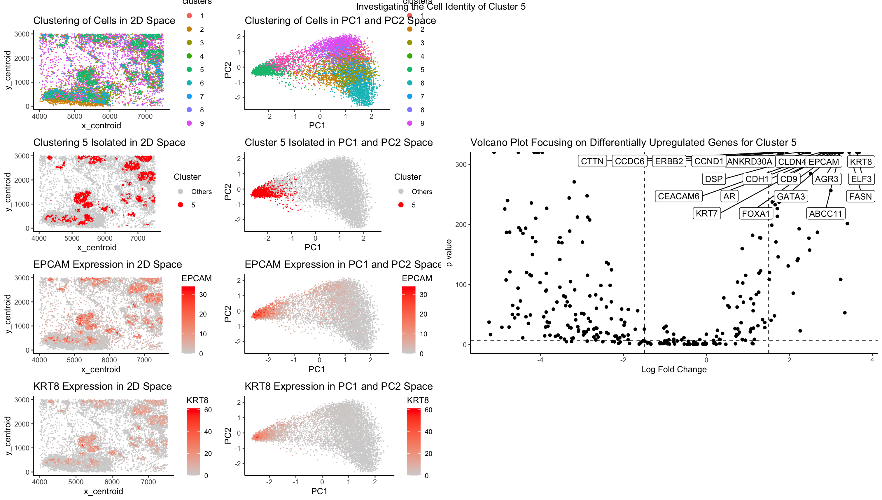
After performing kmeans clustering on my dataset, I randomly decided on investigating cluster 5 of my kmeans clustering. After a thorough analysis, I have concluded that this cluster is likely an epithelial cell cluster. This was concluded via identifying significantly upregulated genes that distinguish cluster 5 from other clusters, as demonstrated in the plots that plot the expression of CLDN4 and KRT8. I also took a look at the top 20 significantly upregulated genes specific to cluster 5, and identified several genes that support my conclusion. Utilizing the NIH’s genebank, I was able to identify specific functions or proteins associated with these genes. Some of these genes include AGR3, ANKRD30A, CLDN4, CTTN, EPCAM, KRT7, and KRT8. These genes specifically regulate functions related to epithelial cells, such as CTTN, which organizes the adhesion structures of epithelial cells. Or genes that encode for epithelial cell function, such as EPCAM, which encodes for epithelial cell adhesion molecules on the cell surface.

These evidences support my conclusion that cluster 5 is an epithelial cell cluster. Further validation work should be conducted to verify that this cluster is indeed epithelial cells. However, more work can be done to specifically identify which type of epithelial cells this cluster belongs to by first separating specific epithelial cells and looking at distinct marker genes between the two populations and seeing if this gene set has those genes.

Sources referenced: https://www.ncbi.nlm.nih.gov/gene/4072 (EPCAM) https://www.ncbi.nlm.nih.gov/gene/155465 (AGR3) https://www.ncbi.nlm.nih.gov/gene/91074 (ANKRD30A) https://www.ncbi.nlm.nih.gov/gene/1364 (CLDN4) https://www.ncbi.nlm.nih.gov/gene/2017 (CTTN) https://www.ncbi.nlm.nih.gov/gene/3855 (KRT7) https://www.ncbi.nlm.nih.gov/gene/3856 (KRT8)

library(ggplot2)

## load in data
data <- read.csv('/Users/ryanchan/Desktop/gdv_2023/data/charmander.csv.gz', 
                 row.names = 1)

## isolate position/ gexp
pos <- data[,1:2]
gexp <- data[, 4:ncol(data)]

## filter cells with no gene expression
good.cells <- rownames(gexp)[rowSums(gexp) > 0]
pos <- pos[good.cells,]
gexp <- gexp[good.cells,]

## normalize by making each cell have same total copies of genes and log10 transforming
totgexp <- rowSums(gexp)
mat <- gexp/totgexp
mat <- mat*mean(totgexp)
mat <- log10(mat + 1)

## running PCA first
pcs <- prcomp(mat)

## find optimal PCs for kmeans
plot(1:50, pcs$sdev[1:50], type = 'l')
plot(1:20, pcs$sdev[1:20], type = 'l')
plot(1:10, pcs$sdev[1:10], type = 'l')

## 9 PCS seem to account for a good amount of variance without sacrificing for too much noise

## loop through ks to find optimal k number of centers
ks <- 1:50
opt.pcs <- 9
out.pcs <- sapply(ks, function(k){
  com <- kmeans(pcs$x[,1:opt.pcs], centers=k)
  c(within = com$tot.withinss, between = com$betweenss)
})

## check for best k number of centers
par(mfrow = c(1,2))
plot(ks, out.pcs[1,], type="l")
plot(ks, out.pcs[2,], type="l")
plot(1:20, out.pcs[1, 1:20], type = "l")
plot(1:10, out.pcs[1, 1:10], type = "l")

## identify that the optimal number of k centers is 10
opt.ks.pca <- 10

## set seed for reproducibility
set.seed(0)
com.pca <- kmeans(pcs$x[,1:opt.pcs], centers = opt.ks.pca)
df.pca <- data.frame(pos, clusters = as.factor(com.pca$cluster), gexp, pcs$x[,1:10])
df.pca[1:5,1:5]

## check cluster size to ensure no clusters are too small
pca.cluster.size <- lapply(1:opt.ks.pca,function(c){
  sum(df.pca$clusters == c)
})
pca.cluster.size

## plot all cells in 2D space
spatial.cluster <- ggplot(data = df.pca, aes(x = x_centroid, y = y_centroid, col = clusters)) + 
  geom_point(size = 0.1) + theme_classic() +
  guides(color = guide_legend(override.aes = list(size = 2.5))) +
  labs(title = 'Clustering of Cells in 2D Space')
spatial.cluster


## plot all cells in PCA space
pca.cluster <- ggplot(data = df.pca, aes(x = PC1, y = PC2, col = clusters)) + 
  geom_point(size = 0.1) + theme_classic() + 
  guides(color = guide_legend(override.aes = list(size = 2.5))) +
  labs(title = 'Clustering of Cells in PC1 and PC2 Space')
pca.cluster

## pick cluster 5 to identify and further investigate

## plot cluster 5 in PC space
pca.cluster5 <- ggplot(data = df.pca, aes(x = PC1, y = PC2, col = clusters == 5)) + 
  geom_point(size = 0.1) + theme_classic() + 
  guides(color = guide_legend(override.aes = list(size = 2.5))) +
  labs(title = 'Cluster 5 Isolated in PC1 and PC2 Space') +
  scale_color_manual(name = 'Cluster',
                     values = c('lightgrey', 'red'),
                     labels = c('Others', '5'))
pca.cluster5


## plot cluster 5 in 2d space
s.cluster5 <- ggplot(data = df.pca, aes(x = x_centroid, y = y_centroid, col = clusters == 5)) + 
  geom_point(size = 0.1) + theme_classic() +
  guides(color = guide_legend(override.aes = list(size = 2.5))) +
  labs(title = 'Clustering 5 Isolated in 2D Space') +
  scale_color_manual(name = 'Cluster',
                   values = c('lightgrey', 'red'),
                   labels = c('Others', '5'))
s.cluster5

## isolate cluster 5 and all other cells
cluster5 <- df.pca[df.pca$clusters == 5, ]
cluster.other <- df.pca[df.pca$clusters != 5, ]
dim(cluster5)
dim(cluster.other)

## identify differentially expressed genes via wilcox.test
diff.genes <- sapply(colnames(gexp), function(g){ 
  wilcox.test(gexp[row.names(cluster5), g], gexp[row.names(cluster.other), g])$p.value  
})

## calculate fold change compared to mean expression of all other cells
logfc <- sapply(colnames(gexp), function(g) {
  log2(mean(gexp[row.names(cluster5), g])/mean(gexp[row.names(cluster.other), g]))
})
df <- data.frame(logfc, pv=-log10(diff.genes))

## only identify upregulated genes by using alternative = greater
up.genes <- sapply(colnames(gexp), function(g){
  wilcox.test(gexp[row.names(cluster5), g], gexp[row.names(cluster.other), g], alternative = 'greater')$p.value
})

## isolate top 20 upregulated genes
ranked.up.genes <- sort(up.genes, decreasing = FALSE)
twenty.up <- ranked.up.genes[1:20]
twenty.up


library(ggrepel)

## create volcano plot to focus on upregulated genes
p.volcano <- ggplot(df) + geom_point(aes(x = logfc, y = pv)) +
  geom_vline(xintercept = -1.5, linetype = 'dashed') + 
  geom_vline(xintercept = 1.5, linetype = 'dashed') + 
  geom_hline(yintercept = 6, linetype = 'dashed') +
  geom_label_repel(data= df[names(twenty.up),],
            aes(x = logfc, y = pv, label = names(twenty.up)), max.overlaps = 35) +
  theme_classic() + 
  labs(title = 'Volcano Plot Focusing on Differentially Upregulated Genes for Cluster 5',
       x = 'Log Fold Change', y = 'p value')
p.volcano  

## will validate some of these genes via literature search

## plot some of the upregulated genes in 2d and PC space
install.packages('dplyr')
library(dplyr)
p.cldn4 <- ggplot(data = df.pca %>%
                    arrange(CLDN4)
                  , aes(x = PC1, y = PC2, col = CLDN4)) +
  geom_point(size = 0.1) + theme_classic() + 
  scale_color_gradient(low = 'lightgrey', high = 'red') +
  labs(title = 'CLDN4 Expression in PC1 and PC2 Space')
p.cldn4

s.cldn4 <- ggplot(data = data %>% arrange(CLDN4), aes(x = x_centroid, y = y_centroid, col = CLDN4)) +
  geom_point(size = 0.1) + theme_classic() + 
  scale_color_gradient(low = 'lightgrey', high = 'red') +
  labs(title = 'CLDN4 Expression in 2D Space')
s.cldn4

p.krt8 <- ggplot(data = df.pca %>% arrange(KRT8), aes(x = PC1, y = PC2, col = KRT8)) +
  geom_point(size = 0.1) + theme_classic() + 
  scale_color_gradient(low = 'lightgrey', high = 'red') + 
  labs(title = 'KRT8 Expression in PC1 and PC2 Space')
p.krt8

s.krt8 <- ggplot(data = data %>% arrange(KRT8), aes(x = x_centroid, y = y_centroid, col = KRT8)) +
  geom_point(size = 0.1) + theme_classic() + 
  scale_color_gradient(low = 'lightgrey', high = 'red') + 
  labs(title = 'KRT8 Expression in 2D Space')
s.krt8

p.epcam <- ggplot(data = df.pca %>% arrange(EPCAM), aes(x = PC1, y = PC2, col = EPCAM)) +
  geom_point(size = 0.1) + theme_classic() + 
  scale_color_gradient(low = 'lightgrey', high = 'red') + 
  labs(title = 'EPCAM Expression in PC1 and PC2 Space')
p.epcam

s.epcam <- ggplot(data = data %>% arrange(EPCAM), aes(x = x_centroid, y = y_centroid, col = EPCAM)) +
  geom_point(size = 0.1) + theme_classic() + 
  scale_color_gradient(low = 'lightgrey', high = 'red') + 
  labs(title = 'EPCAM Expression in 2D Space')
s.epcam

library(gridExtra)

lay <- rbind(c(1,2,NA,NA),
             c(3,4,9,9),
             c(5,6,9,9),
             c(7,8,NA,NA))
grid.arrange(spatial.cluster, pca.cluster,
             s.cluster5, pca.cluster5,
             s.epcam, p.epcam,
             s.krt8, p.krt8,
             p.volcano
             , layout_matrix = lay, top = 'Investigating the Cell Identity of Cluster 5')

## Sources I used for this assignment:
## panel arrangement: https://cran.r-project.org/web/packages/gridExtra/vignettes/arrangeGrob.html
## controlling order of points on plots: https://stackoverflow.com/questions/15706281/controlling-the-order-of-points-in-ggplot2
## text repel: https://www.r-bloggers.com/2016/01/repel-overlapping-text-labels-in-ggplot2/
## labeling on scatter plot: https://stackoverflow.com/questions/15015356/how-to-do-selective-labeling-with-ggplot-geom-point