Description of HW5

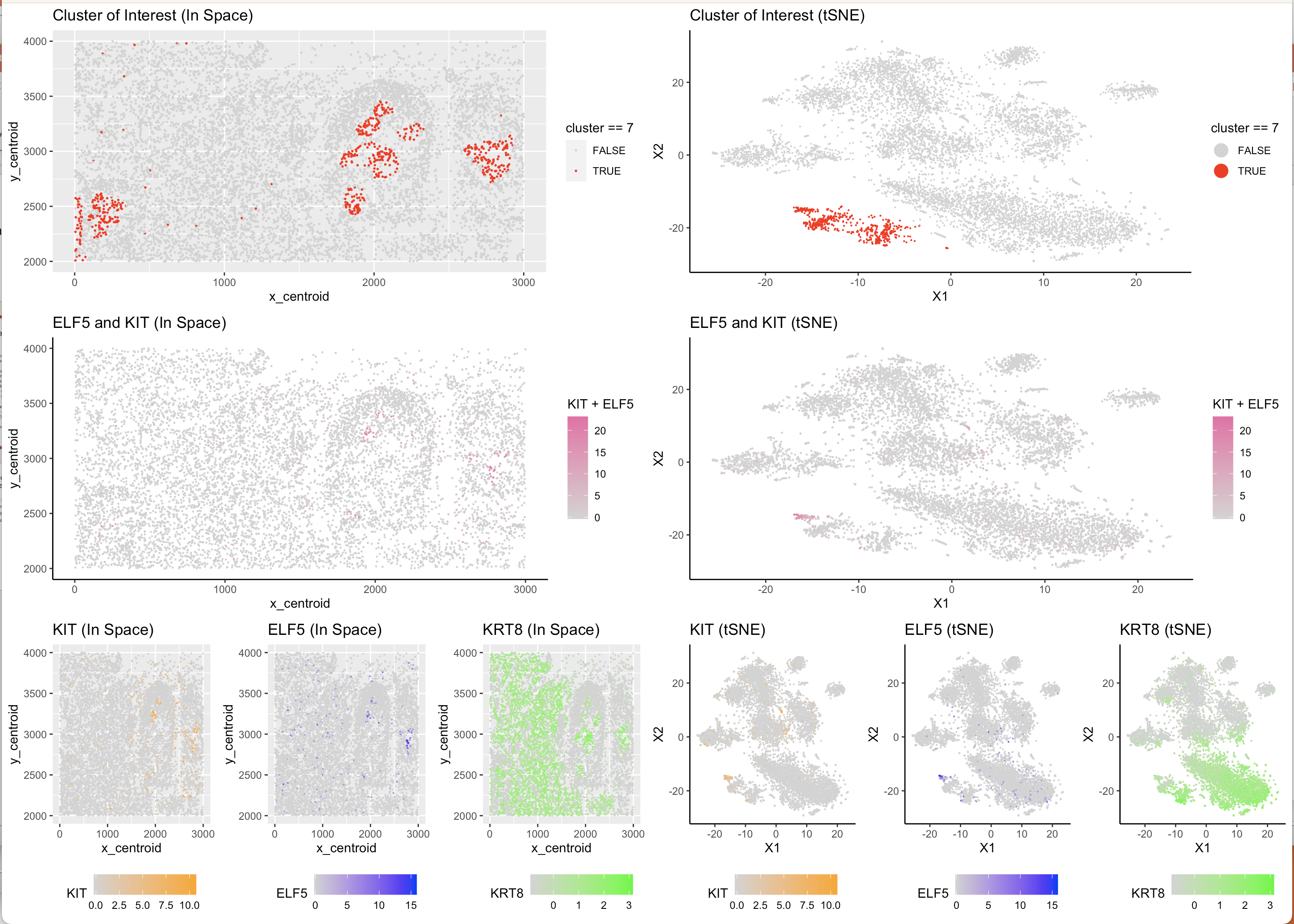
In order to determine cell type from cell cluster, I aimed to find particular genes which are both highly specific to one type of breast cell and also present in the data set. After cross-referencing the genes mentioned in “Profiling human breast epithelial cells using single cell RNA sequencing identifies cell diversity”, I found that KRT8 is a gene that is expressed in Luminal Breast Tissue and was present in the data set. Narrowing down further, ELF5 and KIT are two genes which are specific markers of Luminal Secretory Breast Cells and were present in the data set, this was also confirmed by the paper “A single-cell atlas of the healthy breast tissues reveals clinically relevant clusters of breast epithelial cells” . Using this information, on two levels of specificity, I plotted gene expression levels of these 3 genes on the tSNE Reduced Space and kmeans-clustered cell data and found a pattern. KRT8 was more highly expressed across a larger amount of cells which is to be expected given that is common across the entire subgroup of Luminal cells, both ELF5 and KIT were most highly concentrated in just one of the kmeans clusters which also appeared to be further away in reduced space that many of the other clusters. From there, it was clear that this cluster was likely to be the sub-sub group of Luminal Secretory cells due to the co-expression of KRT8 (indicating that it is a Luminal cell) and ELF5 and KIT which provide additional specificty as markers for only Secretory cells. Using a Wilcox test, I confirmed that all 3 of the genes are differentially upregulated in the cluster of interest (in this case cluster 7) and from that concluded that cluster 7 represents the cell type of Luminal Secretory cells.
Sources:
“Profiling human breast epithelial cells using single cell RNA sequencing identifies cell diversity”: https://www.ncbi.nlm.nih.gov/pmc/articles/PMC5966421/ “A single-cell atlas of the healthy breast tissues reveals clinically relevant clusters of breast epithelial cells”: https://www.sciencedirect.com/science/article/pii/S2666379121000355 “The Ets transcription factor Elf5 specifies mammary alveolar cell fate” - not mentioned in the description, but this paper indicates that the presence of ELF5 is important and differentiating luminal progenitor cells for secretion/lactation https://www.ncbi.nlm.nih.gov/pmc/articles/PMC2259028/
Code:
1
2
3
4
5
6
7
8
9
10
11
12
13
14
15
16
17
18
19
20
21
22
23
24
25
26
27
28
29
30
31
32
33
34
35
36
37
38
39
40
41
42
43
44
45
46
47
48
49
50
51
52
53
54
55
56
57
58
59
60
61
62
63
64
65
66
67
68
69
70
71
72
73
74
75
76
77
78
79
80
81
82
83
84
85
86
87
88
89
90
91
92
93
94
95
96
97
98
99
100
101
102
103
104
105
106
107
108
109
110
111
data <- read.csv('~/Desktop/GDV/GDV23/bulbasaur.csv.gz')

#### initialization ####
#source: in-class by Prof. Fan (1/27)
pos <- data[,2:3]
area <- data[,4]
gexp <- as.matrix(data[,5:ncol(data)])

#### scale data  ####
# (source: in class)
mat <- log10(gexp+1)
mat <- scale(mat)

#### run tSNE and kmeans (cluster plots are down below, elbow at k = 10) ####
emb <- Rtsne::Rtsne(mat, perplexity = 100, check = FALSE)
com <- kmeans(emb$Y, centers = 10)

####plots ####
#source: previous homeworks, in class
# source for legend placement: https://statisticsglobe.com/add-common-legend-to-combined-ggplot2-plots-in-r/
##data exploration for differential gene expression can be found in section "genes of interest"
library(ggplot2)
df <- data.frame(pos, emb$Y, com=as.factor(com$cluster), KIT = mat[, 'KIT'], ELF5 = mat[,'ELF5'], KRT8 = mat[,'KRT8'])
# source: legend size: https://www.geeksforgeeks.org/control-size-of-ggplot2-legend-items-in-r/
p1 <- ggplot(df, aes(x = X1, y = X2, col=com)) + geom_point(size = 0.1) +
  theme_classic() + guides(color = guide_legend(override.aes = list(size = 5)))

pKIT_tsne <- ggplot(df, aes(x = X1, y = X2, col= KIT)) + geom_point(size = 0.1) +
  theme_classic()  + scale_color_continuous(low = 'lightgrey', high= 'orange') +
  ggtitle('KIT (tSNE) ') +
  theme(legend.position = "bottom")

pKIT_space <- ggplot(df, aes(x = x_centroid, y = y_centroid, col = KIT)) + geom_point(size = .1) +
  scale_color_continuous(low = "lightgrey", high = "orange") + ggtitle("KIT (In Space)") +
  theme(legend.position = "bottom")

pELF5_tsne <- ggplot(df, aes(x = X1, y = X2, col= ELF5)) + geom_point(size = 0.1) +
  theme_classic()  + scale_color_continuous(low = 'lightgrey', high='blue') +
  ggtitle('ELF5 (tSNE)') +
  theme(legend.position = "bottom")

pELF5_space <- ggplot(df, aes(x = x_centroid, y = y_centroid, col = ELF5)) + geom_point(size = .1) +
  scale_color_continuous(low = "lightgrey", high = "blue") + ggtitle("ELF5 (In Space)")+
  theme(legend.position = "bottom")

pBOTH_tsne <- ggplot(df, aes(x = X1, y = X2, col= KIT + ELF5)) + geom_point(size = 0.2) +
  theme_classic()  + scale_color_continuous(low = 'lightgrey', high='hotpink2') +
  ggtitle('ELF5 and KIT (tSNE)')

pBOTH_space <- ggplot(df, aes(x = x_centroid, y = y_centroid, col= KIT + ELF5)) + geom_point(size = 0.2) +
  theme_classic()  + scale_color_continuous(low = 'lightgrey', high='hotpink2') +
  ggtitle('ELF5 and KIT (In Space)')

pKRT8_tsne <- ggplot(df, aes(x = X1, y = X2, col= KRT8)) + geom_point(size = 0.1) +
  theme_classic()  + scale_color_continuous(low = 'lightgrey', high='green') +
  ggtitle('KRT8 (tSNE)')  +
  theme(legend.position = "bottom")

pKRT8_space <- ggplot(df, aes(x = x_centroid, y = y_centroid, col = KRT8)) + geom_point(size = .1) +
  scale_color_continuous(low = "lightgrey", high = "green") + ggtitle("KRT8 (In Space)")+
  theme(legend.position = "bottom")

df2 <- data.frame(pos,emb$Y, cluster = as.factor(com$cluster) )

pCluster_Space <- ggplot(df2, aes(x = x_centroid, y = y_centroid, col = cluster == 7)) + geom_point(size = .3) +
  scale_color_manual(values=c("lightgrey", "red")) + ggtitle("Cluster of Interest (In Space)")

pCluster_tsne<- ggplot(df2, aes(x = X1, y = X2, col= cluster == 7)) + geom_point(size = 0.1) +
  theme_classic() + guides(color = guide_legend(override.aes = list(size = 5))) +
  scale_color_manual(values=c("lightgrey", "red")) + ggtitle('Cluster of Interest (tSNE)')


library(gridExtra)

#source: Gohta's "Running tSNE analysis on genes or PCs"  https://jef.works/genomic-data-visualization-2023/blog/2023/02/06/gaihara1/
lay <- rbind(c(9,9,9,10,10,10),
            c(2,2,2,1,1,1),
            c(6,7,8,3,4,5))
grid.arrange(pBOTH_tsne, pBOTH_space, pKIT_tsne, pELF5_tsne, pKRT8_tsne, pKIT_space, pELF5_space,
             pKRT8_space, pCluster_Space, pCluster_tsne, layout_matrix = lay)


#### testing for differential gene expression for genes of interest (ELF5, KRT8, KIT) ####
## source: in class
cluster.cells <- which(com$cluster == 7)
other.cells <- which(com$cluster != 7)
cells <- c(cluster.cells,other.cells)

out1 <- sapply(colnames(mat), function(g) {
  wilcox.test(mat[cluster.cells, g],
              mat[other.cells, g],
              alternative = 'greater')$p.value
})

diff.up.genes <- names(out1)[out1 < 0.005]
sort(out1[diff.up.genes])
# source: https://www.tutorialkart.com/r-tutorial/r-check-if-specific-item-is-present-in-list/
genes_of_interest = c("ELF5" %in% diff.up.genes, "KRT8" %in% diff.up.genes, 'KIT' %in% diff.up.genes)
#check if genes of interest are upregulated, will print true if in the list of upregulated genes
print(genes_of_interest)


#### find number of clusters, seems to be about 10 from within ss plot ####
ks <- 1:20
 out <- do.call(rbind, lapply(ks, function(k){
   com <- kmeans(emb$Y, centers=k)
   c(within = com$tot.withinss, between = com$betweenss)
 }))

plot(ks, out[,1], type="l")
plot(ks, out[,2], type="l")