Exploration of Spatial Gene Expression

A general idea about the exploration
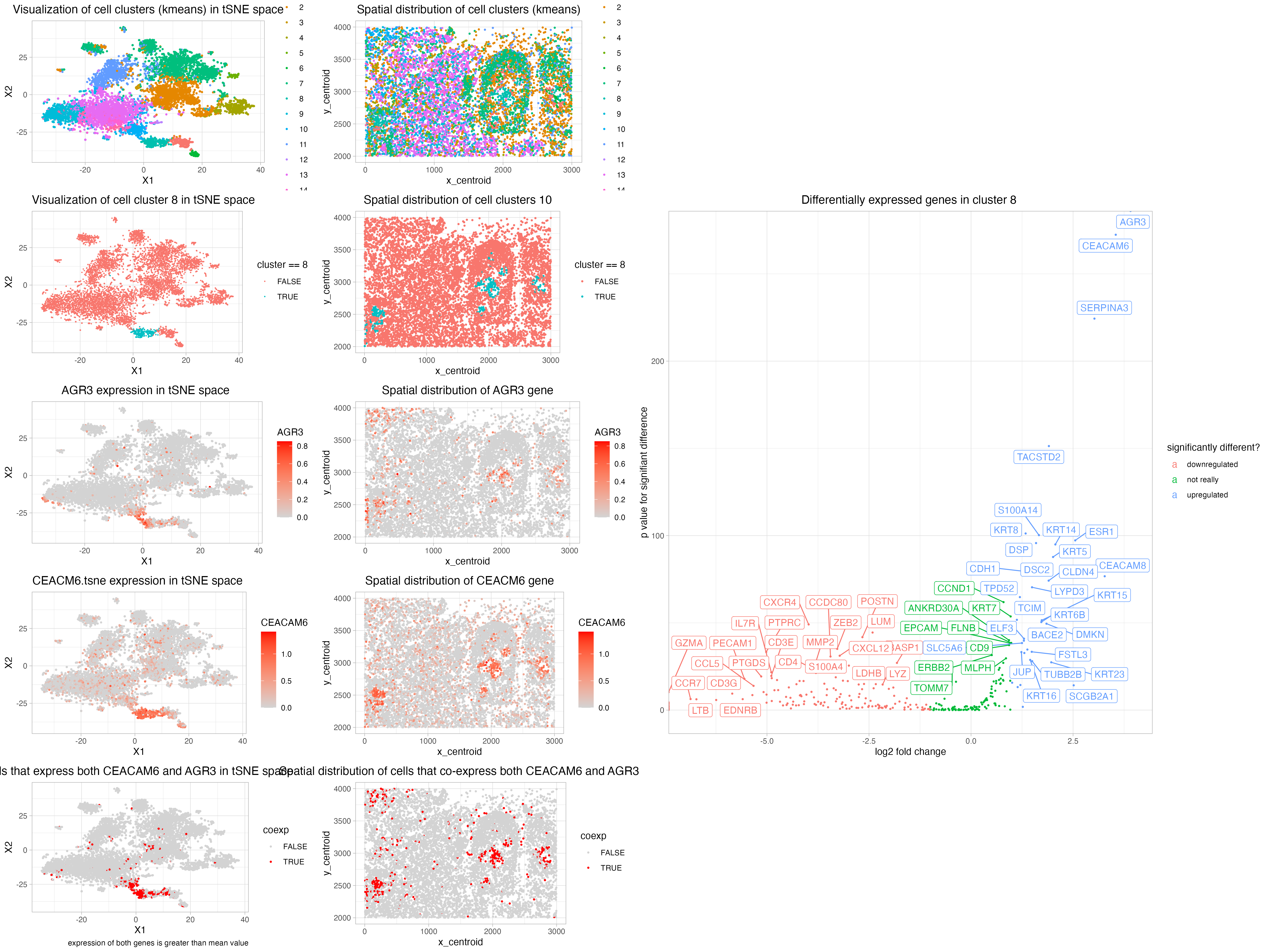
My conclusion about the cell type to be most specific guess would be carcinoma.
I performed log transformation and scale for dimensionality reduction processing and kmeans clustering. From an exploratory plotting of the within cluster variance and eween cluster variance, I found out that the metrics get “better” with more clusters kept. However, for runtime and simplicity concerns, I arbitrarily cut off k value (#cluster) at 15. After an exploratory plotting of what each of the 15 clusters look like in tissue space, I focused on cluster 8 for further exploration. Cluster 8 has a relatively well-defined “spatial” pattern: the cells usually are at the center of some round structure, which reminds me of some medulla. In contrast, multiple clusters are diffused through space.
From a log2 fold change and wilcox ranked sum test exploration, my most significantly expressed genes include: AGR3, CEACAM6, SERPINA3, TACSTD2, KRT8, S100A14, ESR1, DSP, KRT14, KRT5, DSC2, CDH1, CEACAM8, CLDN4.
It is also worth noticing that after log2 fold change plotting, CXCR4, POSTN, LUM seem to be signifiantly downregulated.
GeneCards https://www.genecards.org AGR3: endoplasmic reticulum (ER) protein. expressed in ciliated airway epithelial cells. This gene is also over-expressed in breast, ovarian, and prostrate cancers
NCBI: https://www.ncbi.nlm.nih.gov/gene/4680 CEACAM6: widely used as tumor markers in serum immunoassay determinations of carcinoma. Protein acts as a receptor for adherent-invasive E. coli adhesion to the surface of ileal epithelial cells in patients with Crohn’s disease. This gene is clustered with genes and pseudogenes of the cell adhesion molecules. Biased expression in colon (RPKM 147.4), lung (RPKM 142.2) and 9 other tissues.
NCBI: https://www.ncbi.nlm.nih.gov/gene/12 SERPINA3 not really interesting
GENECards: https://www.genecards.org/cgi-bin/carddisp.pl?gene=TACSTD2 TACSTD2: carcinoma-associated antigen
NCBI: https://www.ncbi.nlm.nih.gov/gene/3856#gene-expression KRT8: Biased expression in colon (RPKM 581.2), small intestine (RPKM 486.1
NCBI: https://www.ncbi.nlm.nih.gov/gene/13982 ESR1: estrogen receptor
Hence, my biggest generalization about the cluster 8 cells is that - it is an epithelial cell. If I were to be more specific, I would conclude it to be an carcinoma (epithelial cancer cells). However, from this particular cell type, I could not make a confident generalization about the location, as it can be anywhere from breast, colon, gallblader, to lung.
I do not see enough overlapping evidence from this breast cancer scRNA profiling paper (https://www.ncbi.nlm.nih.gov/pmc/articles/PMC9044823/) per the gene names appeared in the figures. Nor this paper on non-small lung cancer. (https://www.nature.com/articles/s41467-021-22801-0)
Thanks Gary for volcano plot and final arrangement help!
In addition, referenced this for ideas about the legend (https://www.datanovia.com/en/blog/ggplot-legend-title-position-and-labels/).
Most ideas are from lecture notes ++ reading R documentation.
1
2
3
4
5
6
7
8
9
10
11
12
13
knitr::opts_chunk$set(echo = TRUE)


library(ggplot2)
library(gridExtra)
library(dplyr)
library(ggrepel) ## install.packages("ggrepel")
library(gganimate)
library(Rtsne)
library(magick)

data <- read.csv("~/Desktop/GitHub_Repo/genomic-data-visualization-notes/project/bulbasaur.csv",row.names = 1)
1
2
3
4
5
6
7
8
9
10
11
12
13
14
15
16
17
18
19
20
21

pos <- data[,1:2]
gexp <- data[, 4:ncol(data)]

# screen for ~moderately expressing cells
good.cells <- rownames(gexp)[rowSums(gexp) > 10]
pos <- pos[good.cells,]
gexp <- gexp[good.cells,]

# into a proportion
# note: lose information about gene abundance (absolute counts)
# expand to a scaled value
totgexp <- rowSums(gexp)
mat <- gexp/totgexp
# normalize
mat <- mat*median(totgexp)
# log transformation
mat <- log10(mat + 1)
# scaling variance
mat.scaled <- scale(mat)
1
2
3
4
5
6
7
8
9
10
11
12
set.seed(0)

emb <- Rtsne::Rtsne(mat.scaled)

pcs <- prcomp(mat.scaled)

top.10.pcs <- data.frame(pcs$x[,1:10])

# plot(pcs$sdev[1:100]/sum(pcs$sdev)*100, xlab = "PC",
#      ylab = "Proportion of Variance Explained"
#      )
1
2
3
4
5
6
7
8
9
results <- do.call(rbind, lapply(seq_len(20), function(k) {
  out <- kmeans(mat.scaled, centers=k, iter.max = 20)
  c(out$tot.withinss, out$betweenss)
}))
par(mfrow=c(1,2))

plot(seq_len(20), results[,1], main='tot.withinss')
plot(seq_len(20), results[,2], main='betweenss')
From the above plotting, it seems that k should be bigger if possible. For runtime concerns, cut off at 15 clusters.
1
2
3
4
5
6
7
8
9
10
11
12
13
14
15
16
17
18
19
20
21
22
23
24
25
26
27
28
set.seed(0)
com <- kmeans(mat.scaled, centers=15)

cluster <- com$cluster

tsne.df <- data.frame(pos,
                      emb$Y,
                      cluster = as.factor(cluster))


all.cluster.tSNE <- ggplot(tsne.df,
       aes (x =X1, y = X2, col = cluster)) +
    geom_point(size = 0.5) +
    theme_light() +
    ggtitle("Visualization of cell clusters (kmeans) in tSNE space") +
    theme(plot.title = element_text(hjust = 0.5))

all.cluster.tSNE

all.cluster.space <- ggplot(tsne.df,
       aes (x =x_centroid, y = y_centroid, col = cluster)) +
    geom_point(size = 0.5) +
    theme_light() +
    ggtitle("Spatial distribution of cell clusters (kmeans)") +
    theme(plot.title = element_text(hjust = 0.5))

all.cluster.space
1
2
3
4
5
6
7
8
9
10
11
12
13
14
15
16
17
18
19
20
21
22
23
24
25
26
27
28
29
30

par(mfrow = c(4,dim(com$centers)[1]/4))

loop_plot <- lapply(c(1:dim(com$centers)[1]), function(g) {
    fig <- ggplot(tsne.df, aes(x = x_centroid, y = y_centroid, col = cluster == g)) +
        geom_point(size = 0.1) +
        labs(title = paste("cluster number", g))
    })

loop_plot

cluster8.tSNE <- ggplot(tsne.df, aes(x = X1, y = X2, col = cluster == 8)) +
    geom_point(size = 0.1) +
    ggtitle("Visualization of cell cluster 8 in tSNE space") +
    theme(plot.title = element_text(hjust = 0.5)) +
    theme_light()

cluster8.tSNE


cluster8.space <- ggplot(tsne.df,
       aes (x =x_centroid, y = y_centroid, col = cluster == 8)) +
    geom_point(size = 0.5) +
    theme_light() +
    ggtitle("Spatial distribution of cell clusters 10") +
    theme(plot.title = element_text(hjust = 0.5))

cluster8.space
Cluster 8 is cute - it seems to line the medulla part of whatever structure in sapce
Notice that here I do not use the scaled gene transformation (mat.scale) because in that case, trivial genes would universaly be 0 in the diffgexp matrix
I’ve also tried several other clusters - cluster 10 for exmaple, but it is really diffused across space and the significant differentially expressed genes have ~8 genes with p values == 0
1
2
3
4
5
6
7
8
9
10
11
12
13
cluster.of.interest.df <- data.frame(pos,
                                  emb$Y,
                                  cluster = as.factor(cluster),
                                  target = cluster == 8)

diffgexp <- sapply(colnames(mat), function(g) {
    cluster8 <- names(which(cluster == 8)) # created a variable named cluster well ahead
    ctother <- (names(which(cluster!=8)))
    wilcox.test(mat[cluster8, g],
                mat[ctother,g],
                alternative = "two.sided" )$p.value})

head(sort(diffgexp), n = 20)
1
2
3
4
5
6
7

log2fc <- sapply(colnames(mat), function(g) {
    cluster8 <- names(which(cluster == 8))
    ctother <- names(which(cluster!=8))
    log2(mean(mat[cluster8,g])/mean(mat[ctother,g]))
})
1
2
3
4
5
6
7
8
9
10
11
12
13
14
15
16
17
18
19
20
21
22
23
24
25
26
27
28
29
30
31
32
33
34
35
36

log2fc.df <- data.frame(log2fc, pval = log10(diffgexp))

regulated <- apply(log2fc.df, 1, function(g) {
    if (g['pval'] < 0.01 & g['log2fc']> 1) {
    status <- 1 # upregulated
} else if (g['pval'] < 0.01 &g['log2fc']< -1 ) {
    status <- -1 # downregulated
} else {
    status <- 0 # not significant
}
    #status
    #print(g['pval'])
    }
)

log2fc.df <- log2fc.df %>% cbind(regulated)
log2fc.df$pval <- -log2fc.df$pv

log2fc.plot <- ggplot(log2fc.df,
       aes(y=pval,
           x=log2fc,
           col=as.factor(regulated))) +
    geom_point(size = 0.5) +
    ggrepel::geom_label_repel(label=rownames(log2fc.df),
                              max.overlaps = 30) +
    #scale_color_manual(values = c("blue","lightgrey","red")) +
    scale_color_discrete(name = "significantly different?", labels = c("downregulated", "not really", "upregulated")) +
    ggtitle("Differentially expressed genes in cluster 8 ") +
    xlab("log2 fold change") +
    ylab("p value for signifiant difference") +
    theme_light() +
    theme(plot.title = element_text(hjust = 0.5))


log2fc.plot
1
2
3
4
5
6
7
8
9
10
11
12
13
14
15
16
17
18
19
20
21
22
23
24

tsne.df$AGR3 <- mat$AGR3
AGR3.tsne <- ggplot(tsne.df,
                    aes(x = X1, y = X2, col = AGR3)) +
    geom_point(size = 0.5) +
    scale_color_gradient(low = 'lightgrey',high = 'red') +
    ggtitle("AGR3 expression in tSNE space ") +
    theme_light() +
    theme(plot.title = element_text(hjust = 0.5))


AGR3.tsne


AGR3.space <- ggplot(tsne.df,
       aes (x =x_centroid, y = y_centroid, col = AGR3)) +
    geom_point(size = 0.5) +
    scale_color_gradient(low = 'lightgrey',high = 'red') +
    theme_light() +
    ggtitle("Spatial distribution of AGR3 gene") +
    theme(plot.title = element_text(hjust = 0.5))

AGR3.space
which is nice! As I can see that AGR3 expression is ~high in cluster 8 essentially.
1
2
3
4
5
6
7
8
9
10
11
12
13
14
15
16
17
18
19
20
21
22
23
24

tsne.df$CEACAM6 <- mat$CEACAM6
CEACAM6.tsne <- ggplot(tsne.df,
                    aes(x = X1, y = X2, col = CEACAM6)) +
    geom_point(size = 0.5) +
    scale_color_gradient(low = 'lightgrey',high = 'red') +
    ggtitle("CEACM6.tsne expression in tSNE space ") +
    theme_light() +
    theme(plot.title = element_text(hjust = 0.5))


CEACAM6.tsne


CEACAM6.space <- ggplot(tsne.df,
       aes (x =x_centroid, y = y_centroid, col = CEACAM6)) +
    geom_point(size = 0.5) +
    scale_color_gradient(low = 'lightgrey',high = 'red') +
    theme_light() +
    ggtitle("Spatial distribution of CEACM6 gene") +
    theme(plot.title = element_text(hjust = 0.5))

CEACAM6.space
CEACAM6 is generally a good predictor but not essentially
1
2
3
4
5
6
7
8
9
10
11
12
13
14
15
16
17
18
19
20
21
22
23
24
25
26

# just a rough idea
tsne.df$coexp <- (mat$CEACAM6 > mean(mat$CEACAM6)) & (mat$AGR3 > mean(mat$AGR3))

co.tsne <- ggplot(tsne.df,
                    aes(x = X1, y = X2, col = coexp)) +
    geom_point(size = 0.5) +
    scale_color_manual(values = c('lightgrey','red')) +
    ggtitle("cells that express both CEACAM6 and AGR3 in tSNE space ") +
    theme_light() +
    theme(plot.title = element_text(hjust = 0.5)) +
    labs(caption = "expression of both genes is greater than mean value")


co.tsne


co.space <- ggplot(tsne.df,
       aes (x =x_centroid, y = y_centroid, col = coexp)) +
    geom_point(size = 0.5) +
     scale_color_manual(values = c('lightgrey','red')) +
    theme_light() +
    ggtitle("Spatial distribution of cells that co-express both CEACAM6 and AGR3 ") +
    theme(plot.title = element_text(hjust = 0.5))

co.space
1
2
3
4
5
6
7
8
9
10
11
12
13
14
15
16
17

final.plot <- arrangeGrob(all.cluster.tSNE,all.cluster.space,
                           cluster8.tSNE,cluster8.space,
                           AGR3.tsne,AGR3.space,
                           CEACAM6.tsne,CEACAM6.space,
                           co.tsne,co.space,
                           log2fc.plot,
                          layout_matrix = rbind(c(1,2,NA,NA),
                                                c(3,4,11,11),
                                                c(5,6,11,11),
                                                c(7,8,11,11),
                                                c(9,10,NA,NA)))
                          #title = "Exploration of Spacial Gene Expression ")
ggsave(file = "final.png",
       final.plot,
       width = 20,
       height = 15)