Identification of two Cell Clusters

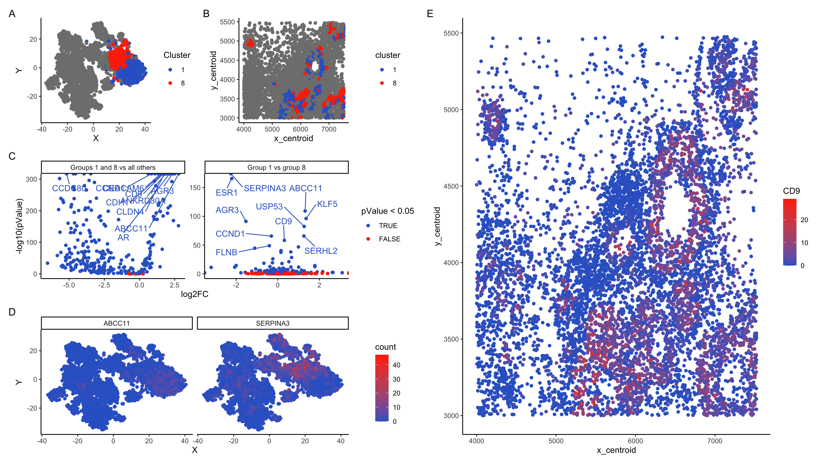
In my plots, I am looking at cell clusters 1 and 8. These clusters separate strongly from the other cells along PC1 and remain close together on t-SNE projections. In t-SNE projections on PCA, cells from these clusters intermix.
Panel B shows that these cells are typically co-localized in ring-like structures. The DGE analysis in panel C supports that these cells are strongly distinct from the surrounding tissue. Comparison of gene expression between group 1 and 8 vs all other cells shows that almost all genes are differentially expressed. Comparison between groups 1 and 8 show that overall most genes are not differentially expressed, but a subset of genes show significantly different expression patterns between the two clusters. Together, this data supports the notion that groups 1 and 8 are two closely-related cell types that are strongly different from the surrounding tissues.
Pulling the top 10 candidate differentially expressed genes between (1 and 8) vs (all other clusters) gives me: “ABCC11”, “AGR3”, “ANKRD30A”, “AR”, “CCDC80”, “CCND1”, “CD9”, “CDH1”, “CEACAM6”, “CLDN4”. A number of these are intriguing. A number of these are intriguing and suggest that clusters 1 and 8 represent breast cancer tumor tissue:
- CCDC80 has association with inhibition of breast cancer cells (Pei et al 2018). It is significantly down-regulated in clusters 1 + 8
- ABCC11 is associated with breast cancert (Ota et al 2010)
- AGR3 is a breast cancer marker gene (Garczyk et al 2015)
- CLDN4 is associated with breast cancer (Abd-Elazeem et al 2015)
and so on. There are plenty of breast cancer-associated genes in these top hits, and the really large-scale global gene expression changes also are consistent with these being cancer cells.
Distinguishing clusters 1 and 8 is harder. Differential genes include as top hits: “SERPINA3”, “ESR1”, “ABCC11”, “KLF5”, “AGR3”, “USP53”, “SERHL2”, “CCND1”, “CD9”, “FLNB”. Most of these have strong associations with breast cancer, but I’m not able to find sources distinguishing cell types based on these markers.
Papers Consulted:
Pei G, Lan Y, Lu W, Ji L, Hua ZC. The function of FAK/CCDC80/E-cadherin pathway in the regulation of B16F10 cell migration. Oncol Lett. 2018 Oct;16(4):4761-4767. doi: 10.3892/ol.2018.9159. Epub 2018 Jul 17. PMID: 30214608; PMCID: PMC6126219.
Ota I, Sakurai A, Toyoda Y, Morita S, Sasaki T, Chishima T, Yamakado M, Kawai Y, Ishidao T, Lezhava A, Yoshiura K, Togo S, Hayashizaki Y, Ishikawa T, Ishikawa T, Endo I, Shimada H. Association between breast cancer risk and the wild-type allele of human ABC transporter ABCC11. Anticancer Res. 2010 Dec;30(12):5189-94. PMID: 21187511.
Garczyk S, von Stillfried S, Antonopoulos W, Hartmann A, Schrauder MG, Fasching PA, Anzeneder T, Tannapfel A, Ergönenc Y, Knüchel R, Rose M, Dahl E. AGR3 in breast cancer: prognostic impact and suitable serum-based biomarker for early cancer detection. PLoS One. 2015 Apr 15;10(4):e0122106. doi: 10.1371/journal.pone.0122106. PMID: 25875093; PMCID: PMC4398490.
Abd-Elazeem MA, Abd-Elazeem MA. Claudin 4 expression in triple-negative breast cancer: correlation with androgen receptors and Ki-67 expression. Ann Diagn Pathol. 2015 Feb;19(1):37-42. doi: 10.1016/j.anndiagpath.2014.10.003. Epub 2014 Oct 25. PMID: 25456318.
Other resources:
Looked at patchwork docs here: https://patchwork.data-imaginist.com/articles/guides/annotation.html Stole this color scale: https://stackoverflow.com/questions/54009145/free-colour-scales-in-facet-grid Looked at how to subset repel labels here: https://stackoverflow.com/questions/60815868/how-to-repel-text-in-one-panel-of-facet-wrap and here: https://stackoverflow.com/questions/52397363/r-ggplot2-ggrepel-label-a-subset-of-points-while-being-aware-of-all-points Looked at repel arguments here: https://www.biostars.org/p/487291/
Code:
library(Rtsne)
library(ggplot2)
library(tidyverse)
library(patchwork)
library(ggrepel)
library(reshape)

# Data import and manipulation
data <- read.csv('~/genomic_data_viz/squirtle.csv.gz', row.names = 1)

# Pull out gene expression
gexp <- data[, 4:ncol(data)]

# Remove empty row
totGenes <- rowSums(gexp)
good.cells <- names(totGenes)[totGenes > 0]

gexp_filtered <- gexp[good.cells,]

# Normalize by gene expression
mat <- gexp[good.cells,]/totGenes[good.cells]
mat <- mat * median(totGenes)

# Log scale
mat <- log(mat + 1)
mat <- mat * median(totGenes)

# K-means Clustering

# Finding optimal k
within_ss_list <- c()
for (i in 1:15){
  k <- kmeans(mat, centers=i)
  within_ss_list <- c(within_ss_list, k$tot.withinss)
}

pltDF <- data.frame(k = 1:15, withinSS <- within_ss_list)
ggplot(pltDF, aes(x = k, y = within_ss_list)) +
  geom_point() +
  theme_classic() +
  scale_x_continuous(breaks=seq(1,15,1),labels=seq(1,15,1))

set.seed(0)
k <- kmeans(mat, centers=8)

# PCA and Tsne
set.seed(0)
pc <- prcomp(gexp_filtered)
set.seed(0)
emb <- Rtsne(mat)
set.seed(0)
emb_pca <- Rtsne(pc$x)

# Data manipulation
pc_plot <- as.data.frame(cbind(pc$x[, c("PC1", "PC2")], cluster_method = "PCA", cluster = k$cluster))
pc_plot$cell_name <- row.names(pc_plot)
colnames(pc_plot) <- c("X", "Y", "cluster_method", "Cluster", "cell_name")


emb_plot <- as.data.frame(cbind(emb$Y,cluster_method = "t-SNE", cluster = k$cluster))
emb_plot$cell_name <- row.names(emb_plot)
colnames(emb_plot) <- c("X", "Y", "cluster_method", "Cluster", "cell_name")

emb_pca_plot <- as.data.frame(cbind(emb_pca$Y, cluster_method = "t-SNE on PCA", cluster = k$cluster))
emb_pca_plot$cell_name <- row.names(emb_pca_plot)
colnames(emb_pca_plot) <- c("X", "Y", "cluster_method", "Cluster", "cell_name")

plt_all <- rbind(pc_plot, emb_plot)
plt_all <- rbind(plt_all, emb_pca_plot)

plt_all$X <- as.numeric(plt_all$X)
plt_all$Y <- as.numeric(plt_all$Y)
plt_all$cluster <- as.factor(plt_all$cluster)

##Plotting
ggplot(data = plt_all, aes(x = X, y = Y, color = Cluster)) +
  geom_point() +
  facet_wrap(~cluster_method, scales = "free") +
  theme_classic() +
  scale_color_viridis_d() +
  theme(axis.title.x = element_blank(), axis.title.y = element_blank())

p1 <- ggplot(data = plt_all[plt_all$cluster_method == "t-SNE", ],  aes(x = X, y = Y, color = Cluster == 1)) +
  geom_point() + theme_classic()

p2 <- ggplot(data = plt_all[plt_all$cluster_method == "t-SNE", ],  aes(x = X, y = Y, color = Cluster == 8)) +
  geom_point() + theme_classic()

p3 <- ggplot(data = plt_all[plt_all$cluster_method == "t-SNE on PCA", ],  aes(x = X, y = Y, color = Cluster == 1)) +
  geom_point() + theme_classic()

p4 <- ggplot(data = plt_all[plt_all$cluster_method == "t-SNE on PCA", ],  aes(x = X, y = Y, color = Cluster == 8)) +
  geom_point() + theme_classic()

(p1 + p2) / (p3 + p4)

# testing
cluster1.cells <-  which(k$cluster == 1)
cluster8.cells <- which(k$cluster == 8)
cluster1_and_8.cells <- which(k$cluster == 1 | k$cluster == 8)
other.cells <- which(k$cluster != 1 & k$cluster != 8)


# First, comparing clusters 1+8 against all else
up_1_and_8 <- sapply(colnames(mat), function(g){
  wilcox.test(mat[cluster1_and_8.cells, g],
              mat[other.cells, g],
              alternative = 'two.sided')$p.value

})

diff.up.genes.1_and_8 <- names(up_1_and_8)[up_1_and_8 < (0.05/ncol(mat))]
diff.up.genes.1_and_8
head(sort(up_1_and_8), n=40)


## Final HW Plots

# A panel visualizing your one cluster of interest in reduced dimensional space (PCA, tSNE, etc)
p1 <- ggplot(data = plt_all[plt_all$cluster_method == "t-SNE", ],  aes(x = X, y = Y, color = Cluster)) +
  geom_point() +
  theme_classic() +
  scale_color_manual(values = c("1" = "#3366CC", "8" = "#FF3300"))

p1

# A panel visualizing your one cluster of interest in space
df_area <- data.frame(data[good.cells, 1:3], cluster = as.factor(k$cluster))

p2 <- ggplot(data = df_area, aes(x=x_centroid, y=y_centroid, color = cluster)) +
  geom_point() +
  theme_classic() +
  scale_color_manual(values = c("1" = "#3366CC", "8" = "#FF3300"))

p2

# A panel visualizing multiple differentially expressed genes for your cluster of interest

up_1_and_8
fc_1_and_8 <- sapply(colnames(mat), function(g){
  log2(mean(mat[cluster1_and_8.cells, g])/mean(mat[other.cells, g]))
})

df_volcano <- data.frame(log2FC = fc_1_and_8, pValue = up_1_and_8, comparison = "Groups 1 and 8 vs all others")

g1_8_vs_all <- ggplot(df_volcano, aes(x = log2FC, y = -log10(pValue), color = pValue < 0.05)) +
  geom_point() +
  theme_classic() +
  ggtitle("Groups 1 and 8 vs all others")

diff_1_8 <- sapply(colnames(mat), function(g){
  wilcox.test(mat[cluster1.cells, g],
              mat[cluster8.cells, g],
              alternative = 'two.sided')$p.value
})

fc_1_vs_8 <- sapply(colnames(mat), function(g){
  log2(mean(mat[cluster1.cells, g])/mean(mat[cluster8.cells, g]))
})

df_volcano_1_vs_8 <- data.frame(log2FC = fc_1_vs_8, pValue = diff_1_8, comparison = "Group 1 vs group 8")

df_volcano$gname <- rownames(df_volcano)
df_volcano_1_vs_8$gname <- rownames(df_volcano_1_vs_8)
df_all_volc <- rbind(df_volcano, df_volcano_1_vs_8)
df_all_volc$comparison <- factor(df_all_volc$comparison,
                                 levels = c("Groups 1 and 8 vs all others", "Group 1 vs group 8"))

g1_vs_g8 <- ggplot(df_volcano_1_vs_8, aes(x = log2FC, y = -log10(pValue), color = pValue < 0.05)) +
  geom_point() +
  theme_classic() +
  ggtitle("Group 1 vs group 8")

low_names_1_and_8 <- names(head(sort(up_1_and_8), n=10))
low_names_1_vs_8 <- names(head(sort(diff_1_8), n=10))
low_names <- c(low_names_1_and_8, low_names_1_vs_8)