Validation of cell type clustering via differential gene expression

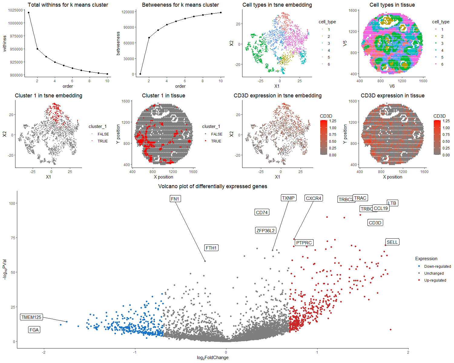
The purpose of this visualization to present the usage of differential gene expression to validate cell type identification in k-means and tsne analysis of the dataset. The quantitative data of gene expression matrix is preprocessed by normalization by total gene counts, and log-scaled. The first row of the figure presented the total withinss and betweeness, and identified six cell clusters are visualized with different color hues encoding different cell types in both tsne space and tissue sample space. I choose to run for 6 clusters, because it is relatively optimal in both total withinss and betweeness plot, with reasonable partition on TSNE plot. The nine clusters all have distinct profiles for top differentially expressed genes, with the typical biomarkers of breast epithelial cells, tumor cells, T cells, B cells, etc. Specifically, here I focus on cluster 1, and argue that it is the T cell population. The first two columns of second row presents the position of cluster 1 in tsne space and tissue space. It forms a coherent cluster in the embedding space, while forms multiple small clusters in real tissue space, which conforms to real physiology that T cell infiltration could happen in multiple sites of the tumor. From the third row of the volcano plot, the genes with more than two fold expression change and having a p value < 0.05 are marked. Among the up-regulated genes, TRBC2, TRAC, LTB, TRBC1, CD74, CD3D, CD37 are all represented markers for the T cell population. TRBC2, TRAC, TRBC1, and CD3D are all T cell receptor subunit genes[1,2,3,4]. LTB stands for lymphotoxin beta, and by its name, usually expresses on surface of lymphocytes including T cells [5]. CD74 could mediate MHC molecule recognition, as well as regulate T-cell development[6]. CD37 is also a leukocyte specific protein that could regulate T cell proliferation[7]. Thus, collectively speaking, it is the most likely that cluster 1 is the T cell population. In the right two columns of the second row, I choose to visualize the quantitative data of CD3D expression on tsne plot and tissue space. Because CD3D has a small p value as well as a high fold change. It is hypothesized that only T cell population should express it, as it is a subunit of T cell receptor. We could see that CD3D expression pattern overlays with cluster 1 but also extends over the region. The correspondence was not as clean as it was for dataset in HW5. It is likely to the mixed of cell types in each spot for the spot-based sequencing strategy. Though the expression of differentially expressed gene failed to perfectly align, the rationale for k means clustering based on total withnss and betweenness, and the abundance for T cell receptor and proliferation marker genes provide reasonble support for the hypothesis that cluster 1 is T cells.

Reference.

[1]https://www.genecards.org/cgi-bin/carddisp.pl?gene=TRBC2&keywords=TRBC2 [2]https://www.genecards.org/cgi-bin/carddisp.pl?gene=TRBC1&keywords=TRBC1 [3]https://www.genecards.org/cgi-bin/carddisp.pl?gene=TRAC&keywords=TRAC [4]https://www.genecards.org/cgi-bin/carddisp.pl?gene=CD3D&keywords=CD3D [5]https://www.genecards.org/cgi-bin/carddisp.pl?gene=LTB&keywords=ltb [6]Su, Huiting et al. “The biological function and significance of CD74 in immune diseases.” Inflammation research : official journal of the European Histamine Research Society … [et al.] vol. 66,3 (2017): 209-216. doi:10.1007/s00011-016-0995-1 [7]van Spriel, Annemiek B et al. “A regulatory role for CD37 in T cell proliferation.” Journal of immunology (Baltimore, Md. : 1950) vol. 172,5 (2004): 2953-61. doi:10.4049/jimmunol.172.5.2953

Code modified from in-class notes and my HW5 code.

Please note that the final output has adjusted canvas size for importing.

Code

library(Rtsne)
library(ggplot2)
library(gridExtra)
library(ggrepel)

data <- read.csv('visium_breast_cancer.csv.gz', row.names = 1)
dim(data)
pos <- data[,1:2]
gexp <- data[,3:ncol(data)]
## normalize
mat <- gexp/rowSums(gexp)
mat <- mat*mean(rowSums(gexp))
mat <- log10(mat + 1)


## make sure you all can run loops
ks <- 1:10
out <- do.call(rbind, lapply(ks, function(k){
  com <- kmeans(mat, centers=k)
  c(within = com$tot.withinss, between = com$betweenss)
}))

df_assess<- data.frame(order = 1:10, withinss = out[,1], betweeness = out[,2])
p1<-ggplot(df_assess,aes(x = order,y = withinss)) + geom_point()+ geom_line()+
  theme_classic() + scale_x_continuous(breaks = c(2,4,6,8,10))+
  theme(plot.title = element_text(hjust = 0.5))+
  ggtitle("Total withinss for k means cluster")
p2<-ggplot(df_assess,aes(x = order,y = betweeness)) + geom_point()+ geom_line()+
  theme_classic() + scale_x_continuous(breaks = c(2,4,6,8,10))+
  theme(plot.title = element_text(hjust = 0.5))+
  ggtitle("Betweeness for k means cluster")
grid.arrange(p1, p2,ncol=1)
#choose k = 6

#perform tsne
set.seed(0) ## for reproducibility
emb <- Rtsne(mat)
com <- kmeans(mat, centers=6) #choose 9 centers as tuned visually from tsne plot

#plot embedding
df <- data.frame(pos, emb$Y, cell_type=as.factor(com$cluster),cluster_1 = (com$cluster == 1))
#plot embedding in tsne space
p3 <- ggplot(df, aes(x = X1, y = X2, col=cell_type)) + 
  geom_point(size = 0.1) +
  ggtitle("Cell types in tsne embedding")+
  theme_classic()+
  theme(plot.title = element_text(hjust = 0.5))
#plot embedding in tissue space
p4 <- ggplot(df, aes(x = V6, y = V5, col=cell_type)) + 
  geom_point(size = 1) + 
  ggtitle("Cell types in tissue")+
  theme_classic()+
  theme(plot.title = element_text(hjust = 0.5))
grid.arrange(p3, p4,ncol=1)

## pick a cluster
## Cluster 1 is likely T cell
cluster_num = 1
cluster.of.interest <- names(which(com$cluster == cluster_num))
cluster.other <- names(which(com$cluster != cluster_num))
## loop through my genes and test each one
genes <- colnames(mat)
pvs <- sapply(genes, function(g) {
  a <- mat[cluster.of.interest, g]
  b <- mat[cluster.other, g]
  wilcox.test(a,b,alternative="two.sided")$p.val
})
head(sort(pvs), n=20)

#plot embedding
df <- data.frame(pos, emb$Y, cell_type=as.factor(com$cluster),cluster_1 = (com$cluster == 1))
#plot embedding in tsne space
p5 <- ggplot(df, aes(x = X1, y = X2, col=cluster_1)) + 
  geom_point(size = 0.1) +
  ggtitle("Cluster 1 in tsne embedding")+
  scale_color_manual(values = c("gray50", "red")) +
  theme_classic()+
  theme(plot.title = element_text(hjust = 0.5))
#plot embedding in tissue space
p6 <- ggplot(df, aes(x = V6, y = V5, col=cluster_1)) + 
  geom_point(size = 1) + 
  ggtitle("Cluster 1 in tissue")+
  scale_color_manual(values = c("gray50", "red")) +
  theme_classic()+
  xlab("X position")+
  ylab("Y position")+
  theme(plot.title = element_text(hjust = 0.5))
grid.arrange(p5, p6,ncol=1)

### calculate a fold change
log2fc <- sapply(genes, function(g) {
  a <- mat[cluster.of.interest, g]
  b <- mat[cluster.other, g]
  log2(mean(a)/mean(b))
})


## volcano plot
deg <- data.frame(pvs, log2fc)
Expression <- apply(deg, 1, function(g) {
  if (g[2] >= log(2) & g[1] <= 0.05) {
    out = "Up-regulated"
  } else if (g[2] <= -log(2) & g[1] <= 0.05) {
    out = "Down-regulated"
  } else {
    out = "Unchanged"
  }
  out
})
deg <- cbind(deg, Expression)

p7 <- ggplot(deg, aes(y=-log10(pvs), x=log2fc)) + 
  geom_point(aes(color = Expression)) +
  xlab(expression("log"[2]*"FoldChange")) + 
  ylab(expression("-log"[10]*"PVal")) +
  scale_color_manual(values = c("dodgerblue3", "gray50", "firebrick3")) +
  guides(colour = guide_legend(override.aes = list(size=1.5))) +
  ggrepel::geom_label_repel(label=rownames(deg))+
  ggtitle("Volcano plot of differentially expressed genes")+
  theme_classic()+
  theme(plot.title = element_text(hjust = 0.5))
p7

#choose to visualize CD3D
df <- cbind(df,CD3D = mat$CD3D)
#plot embedding in tsne space
p8 <- ggplot(df, aes(x = X1, y = X2, col = CD3D)) + 
  geom_point(size = 0.1) +
  ggtitle("CD3D expression in tsne embedding")+
  theme_classic()+
  theme(plot.title = element_text(hjust = 0.5))+
  scale_color_gradient(low = 'gray50', high='red') 
p8
#plot embedding in tissue space
p9 <- ggplot(df, aes(x = V6, y = V5, col=CD3D)) + 
  geom_point(size = 1) + 
  ggtitle("CD3D expression in tissue")+
  theme_classic()+
  xlab("X position")+
  ylab("Y position")+
  theme(plot.title = element_text(hjust = 0.5))+
  scale_color_gradient(low = 'gray50', high='red')
p9

g1 <- grid.arrange(p1, p2, p3, p4,p5,p6,p8,p9, ncol=4)
g2<- grid.arrange(g1, p7,ncol=1)
g2