Identifying an B cell/ Adipocyte Composite Cluster in Visium Dataset

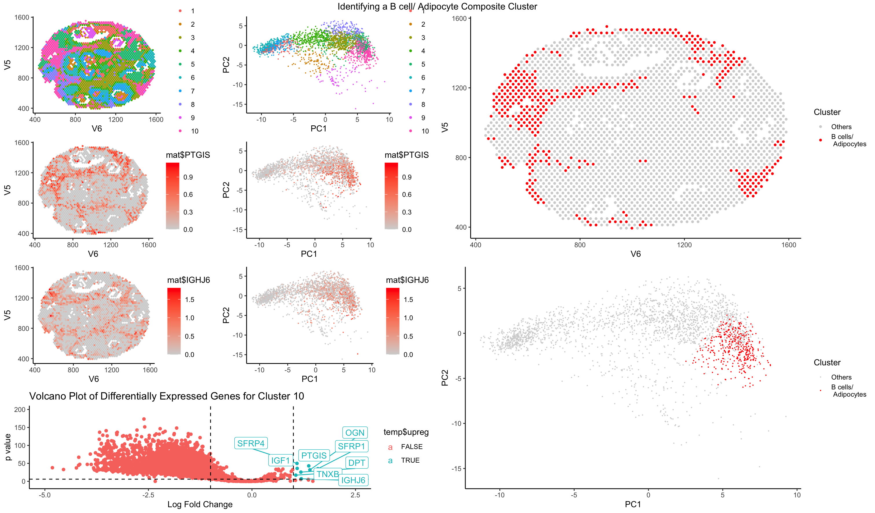
Similar to HW5, I performed kmeans clustering on my normalized dataset. I then went through each of the clusters in spatial representation as well as PC dimensional representation to understand the distribution of the clusters as well as the cluster sizes. I then looked at some top differentially expressed genes, especially upregulated genes. I managed to loop through a few clusters of cells to identify and I decided to present on one of the more interesting populations, a composite cluster of B cells and adipocytes. As a side note, I also identified cluster 1 in the dataset to be a blood cells/ megakaryocyte composite population and cluster 6 as cancer cells.
I arrived to my conclusion for cluster 10 to be a B cell/ adipocyte composite cluster by taking a look at the top differentially expressed genes. It is a mixture of immunoglobulin genes as well as adipogenic related genes such as SFRP4, PTGIS, IGF1, and DPT. The immunoglobulin genes are a clear indicator of B cell function due to the abundance of immunoglobulin genes. However, genes such as SFRP4, which is a part of the WNT signaling pathway, which is closely associated with adipogenesis, PTGIS, which is involved in synthesis of cholesterol, steroids, and other lipids, IGF1 (insulin-like growth factor 1), which is involved in lipogenesis in adpocytes, and DPT, which is broadly expressed in adipose tissue, all point toward the presence of adipocytes in the same cluster. I conclude that this is likely to be a composite cluster rather than an artifact but further analysis will need to be conducted. Some review of how the data was collected will likely be the first step in reviewing whether this is an accurate analysis.
Sources referenced: https://www.ncbi.nlm.nih.gov/pmc/articles/PMC2709272/ (WNT signaling in Adipogenesis) https://www.ncbi.nlm.nih.gov/gene/?term=IGF1 (IGF1) https://www.ncbi.nlm.nih.gov/gene/6424 (SFRP4) https://www.ncbi.nlm.nih.gov/gene/5740 (PTGIS) https://www.ncbi.nlm.nih.gov/gene/28908 (IGKV4)
library(ggplot2)

## load in data
data <- read.csv('/Users/ryanchan/Desktop/gdv_2023/data/charmander.csv.gz',
                 row.names = 1)

## isolate position/ gexp
pos <- data[,1:2]
gexp <- data[, 4:ncol(data)]

## filter cells with no gene expression
good.cells <- rownames(gexp)[rowSums(gexp) > 0]
pos <- pos[good.cells,]
gexp <- gexp[good.cells,]

## normalize by making each cell have same total copies of genes and log10 transforming
totgexp <- rowSums(gexp)
mat <- gexp/totgexp
mat <- mat*mean(totgexp)
mat <- log10(mat + 1)

## running PCA first
pcs <- prcomp(mat)

## find optimal PCs for kmeans
plot(1:50, pcs$sdev[1:50], type = 'l')
plot(1:20, pcs$sdev[1:20], type = 'l')
plot(1:10, pcs$sdev[1:10], type = 'l')

## 9 PCS seem to account for a good amount of variance without sacrificing for too much noise

## loop through ks to find optimal k number of centers
ks <- 1:50
opt.pcs <- 9
out.pcs <- sapply(ks, function(k){
  com <- kmeans(pcs$x[,1:opt.pcs], centers=k)
  c(within = com$tot.withinss, between = com$betweenss)
})

## check for best k number of centers
par(mfrow = c(1,2))
plot(ks, out.pcs[1,], type="l")
plot(ks, out.pcs[2,], type="l")
plot(1:20, out.pcs[1, 1:20], type = "l")
plot(1:10, out.pcs[1, 1:10], type = "l")

## identify that the optimal number of k centers is 10
opt.ks.pca <- 10

## set seed for reproducibility
set.seed(0)
com.pca <- kmeans(pcs$x[,1:opt.pcs], centers = opt.ks.pca)
df.pca <- data.frame(pos, clusters = as.factor(com.pca$cluster), gexp, pcs$x[,1:10])
df.pca[1:5,1:5]

## check cluster size to ensure no clusters are too small
pca.cluster.size <- lapply(1:opt.ks.pca,function(c){
  sum(df.pca$clusters == c)
})
pca.cluster.size

## plot all cells in 2D space
spatial.cluster <- ggplot(data = df.pca, aes(x = x_centroid, y = y_centroid, col = clusters)) +
  geom_point(size = 0.1) + theme_classic() +
  guides(color = guide_legend(override.aes = list(size = 2.5))) +
  labs(title = 'Clustering of Cells in 2D Space')
spatial.cluster


## plot all cells in PCA space
pca.cluster <- ggplot(data = df.pca, aes(x = PC1, y = PC2, col = clusters)) +
  geom_point(size = 0.1) + theme_classic() +
  guides(color = guide_legend(override.aes = list(size = 2.5))) +
  labs(title = 'Clustering of Cells in PC1 and PC2 Space')
pca.cluster

## pick cluster 5 to identify and further investigate

## plot cluster 5 in PC space
pca.cluster5 <- ggplot(data = df.pca, aes(x = PC1, y = PC2, col = clusters == 5)) +
  geom_point(size = 0.1) + theme_classic() +
  guides(color = guide_legend(override.aes = list(size = 2.5))) +
  labs(title = 'Cluster 5 Isolated in PC1 and PC2 Space') +
  scale_color_manual(name = 'Cluster',
                     values = c('lightgrey', 'red'),
                     labels = c('Others', '5'))
pca.cluster5


## plot cluster 5 in 2d space
s.cluster5 <- ggplot(data = df.pca, aes(x = x_centroid, y = y_centroid, col = clusters == 5)) +
  geom_point(size = 0.1) + theme_classic() +
  guides(color = guide_legend(override.aes = list(size = 2.5))) +
  labs(title = 'Clustering 5 Isolated in 2D Space') +
  scale_color_manual(name = 'Cluster',
                   values = c('lightgrey', 'red'),
                   labels = c('Others', '5'))
s.cluster5

## isolate cluster 5 and all other cells
cluster5 <- df.pca[df.pca$clusters == 5, ]
cluster.other <- df.pca[df.pca$clusters != 5, ]
dim(cluster5)
dim(cluster.other)

## identify differentially expressed genes via wilcox.test
diff.genes <- sapply(colnames(gexp), function(g){
  wilcox.test(gexp[row.names(cluster5), g], gexp[row.names(cluster.other), g])$p.value
})

## calculate fold change compared to mean expression of all other cells
logfc <- sapply(colnames(gexp), function(g) {
  log2(mean(gexp[row.names(cluster5), g])/mean(gexp[row.names(cluster.other), g]))
})
df <- data.frame(logfc, pv=-log10(diff.genes))

## only identify upregulated genes by using alternative = greater
up.genes <- sapply(colnames(gexp), function(g){
  wilcox.test(gexp[row.names(cluster5), g], gexp[row.names(cluster.other), g], alternative = 'greater')$p.value
})

## isolate top 20 upregulated genes
ranked.up.genes <- sort(up.genes, decreasing = FALSE)
twenty.up <- ranked.up.genes[1:20]
twenty.up


library(ggrepel)

## create volcano plot to focus on upregulated genes
p.volcano <- ggplot(df) + geom_point(aes(x = logfc, y = pv)) +
  geom_vline(xintercept = -1.5, linetype = 'dashed') +
  geom_vline(xintercept = 1.5, linetype = 'dashed') +
  geom_hline(yintercept = 6, linetype = 'dashed') +
  geom_label_repel(data= df[names(twenty.up),],
            aes(x = logfc, y = pv, label = names(twenty.up)), max.overlaps = 35) +
  theme_classic() +
  labs(title = 'Volcano Plot Focusing on Differentially Upregulated Genes for Cluster 5',
       x = 'Log Fold Change', y = 'p value')
p.volcano

## will validate some of these genes via literature search

## plot some of the upregulated genes in 2d and PC space
install.packages('dplyr')
library(dplyr)
p.cldn4 <- ggplot(data = df.pca %>%
                    arrange(CLDN4)
                  , aes(x = PC1, y = PC2, col = CLDN4)) +
  geom_point(size = 0.1) + theme_classic() +
  scale_color_gradient(low = 'lightgrey', high = 'red') +
  labs(title = 'CLDN4 Expression in PC1 and PC2 Space')
p.cldn4

s.cldn4 <- ggplot(data = data %>% arrange(CLDN4), aes(x = x_centroid, y = y_centroid, col = CLDN4)) +
  geom_point(size = 0.1) + theme_classic() +
  scale_color_gradient(low = 'lightgrey', high = 'red') +
  labs(title = 'CLDN4 Expression in 2D Space')
s.cldn4

p.krt8 <- ggplot(data = df.pca %>% arrange(KRT8), aes(x = PC1, y = PC2, col = KRT8)) +
  geom_point(size = 0.1) + theme_classic() +
  scale_color_gradient(low = 'lightgrey', high = 'red') +
  labs(title = 'KRT8 Expression in PC1 and PC2 Space')
p.krt8

s.krt8 <- ggplot(data = data %>% arrange(KRT8), aes(x = x_centroid, y = y_centroid, col = KRT8)) +
  geom_point(size = 0.1) + theme_classic() +
  scale_color_gradient(low = 'lightgrey', high = 'red') +
  labs(title = 'KRT8 Expression in 2D Space')
s.krt8

p.epcam <- ggplot(data = df.pca %>% arrange(EPCAM), aes(x = PC1, y = PC2, col = EPCAM)) +
  geom_point(size = 0.1) + theme_classic() +
  scale_color_gradient(low = 'lightgrey', high = 'red') +
  labs(title = 'EPCAM Expression in PC1 and PC2 Space')
p.epcam

s.epcam <- ggplot(data = data %>% arrange(EPCAM), aes(x = x_centroid, y = y_centroid, col = EPCAM)) +
  geom_point(size = 0.1) + theme_classic() +
  scale_color_gradient(low = 'lightgrey', high = 'red') +
  labs(title = 'EPCAM Expression in 2D Space')
s.epcam

library(gridExtra)

lay <- rbind(c(1,2,NA,NA),
             c(3,4,9,9),
             c(5,6,9,9),
             c(7,8,NA,NA))
grid.arrange(spatial.cluster, pca.cluster,
             s.cluster5, pca.cluster5,
             s.epcam, p.epcam,
             s.krt8, p.krt8,
             p.volcano
             , layout_matrix = lay, top = 'Investigating the Cell Identity of Cluster 5')

## Sources I used for this assignment:
## panel arrangement: https://cran.r-project.org/web/packages/gridExtra/vignettes/arrangeGrob.html
## controlling order of points on plots: https://stackoverflow.com/questions/15706281/controlling-the-order-of-points-in-ggplot2
## text repel: https://www.r-bloggers.com/2016/01/repel-overlapping-text-labels-in-ggplot2/
## labeling on scatter plot: https://stackoverflow.com/questions/15015356/how-to-do-selective-labeling-with-ggplot-geom-point