Determining Cell Type for Visium Data
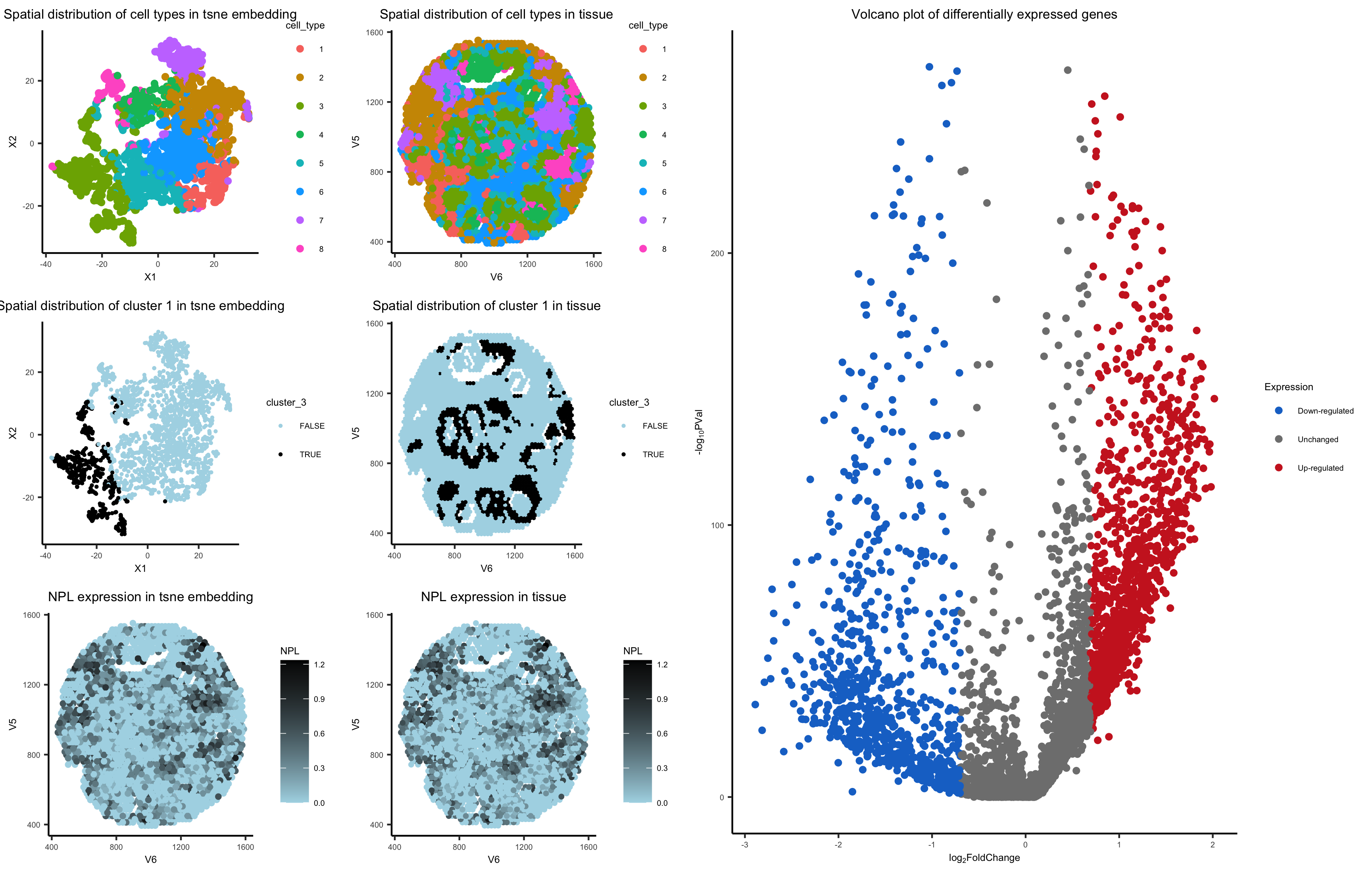
I used kmeans clustering to identify different cell types by looking at clusters in my data. I preproceessed my data by normalizing by total gene count and putting everything on a log scale. I ended up going with 8 clusters because it seemed to categorize and separate everything out pretty well. This number was hard to validate externally because most sources said there were many many types of cells in breast tissue, so I had to use my own judgement. Different sources said different numbers depending on how specific they get.
My NPL gene in cluster 3 is the most upregulated gene. After doing some research, NPL mutations are associated with some heretary breast cancers (source). I think my cell type is actually epithetial cells of breast tissue, because NPL is commonly in renal tubule cells (source), which tend to epithetial (source).
I think this makes sense because choosing the most upregulated gene should have the highest probability of correctly identifying the cell type. The only scenario I could see that not being true is if a gene was upregulated in many many cell types. I did the same approach for analysis as homework 5, so I hope both are correct processes of thinking.
Code
library(Rtsne)
library(ggplot2)
library(gridExtra)
library(ggrepel)
options(ggrepel.max.overlaps = 5)

data <- read.csv('~/Downloads/visium_breast_cancer.csv', row.names = 1)
## pull out gene expression
pos <- data[,1:2]
gexp <- data[, 4:ncol(data)]

good.cells <- rownames(gexp)[rowSums(gexp) > 10]
pos <- pos[good.cells,]
gexp <- gexp[good.cells,]

totgexp <- rowSums(gexp)
mat <- gexp/totgexp
mat <- mat*median(totgexp)
mat <- log10(mat + 1)

#perform tsne
set.seed(0) ## for reproducibility
emb <- Rtsne::Rtsne(mat)
com <- kmeans(mat, centers=8) #4 centers seemed to show good categories without complications

#plot embedding
df <- data.frame(pos, emb$Y, cell_type=as.factor(com$cluster),cluster_3 = (com$cluster == 3))
#plot embedding in tsne space
p1 <- ggplot(df, aes(x = X1, y = X2, col=cell_type)) +
  geom_point(size = 1.5) +
  ggtitle("Spatial distribution of cell types in tsne embedding")+
  theme_classic()+
  theme(plot.title = element_text(size=8, hjust = 0.5), text = element_text(size=6))
p1
#plot embedding in tissue space
p2 <- ggplot(df, aes(x = V6, y = V5, col=cell_type)) +
  geom_point(size = 1.5) +
  ggtitle("Spatial distribution of cell types in tissue")+
  theme_classic()+
  theme(plot.title = element_text(size=8, hjust = 0.5), text = element_text(size=6))
p2
#plot embedding in tsne space
p3 <- ggplot(df, aes(x = X1, y = X2, col=cluster_3)) +
  geom_point(size = 0.5) +
  ggtitle("Spatial distribution of cluster 1 in tsne embedding")+
  scale_color_manual(values = c("lightblue", "black")) +
  theme_classic()+
  theme(plot.title = element_text(size=8, hjust = 0.5), text = element_text(size=6))
p3
#plot embedding in tissue space
p4 <- ggplot(df, aes(x = V6, y = V5, col=cluster_3)) +
  geom_point(size = 0.5) +
  ggtitle("Spatial distribution of cluster 1 in tissue")+
  scale_color_manual(values = c("lightblue", "black")) +
  theme_classic()+
  theme(plot.title = element_text(size=8, hjust = 0.5), text = element_text(size=6))
p4

## pick a cluster
#cluster 3!
cluster_num = 3
cluster.of.interest <- names(which(com$cluster == cluster_num))
cluster.other <- names(which(com$cluster != cluster_num))
## loop through my genes and test each one
genes <- colnames(mat)
pvs <- sapply(genes, function(g) {
  a <- mat[cluster.of.interest, g]
  b <- mat[cluster.other, g]
  wilcox.test(a,b,alternative="two.sided")$p.val
})
names(which(pvs < 1e-8))
head(sort(pvs), n=20)

### calculate a fold change
log2fc <- sapply(genes, function(g) {
  a <- mat[cluster.of.interest, g]
  b <- mat[cluster.other, g]
  log2(mean(a)/mean(b))
})


## volcano plot
deg <- data.frame(pvs, log2fc)
Expression <- apply(deg, 1, function(g) {
  if (g[2] >= log(2) & g[1] <= 0.05) {
    out = "Up-regulated"
  } else if (g[2] <= -log(2) & g[1] <= 0.05) {
    out = "Down-regulated"
  } else {
    out = "Unchanged"
  }
  out
})
deg <- cbind(deg, Expression)

options(repr.plot.width = 8, repr.plot.height =4)
p5 <- ggplot(deg, aes(y=-log10(pvs), x=log2fc)) +
  geom_point(aes(color = Expression)) +
  xlab(expression("log"[2]*"FoldChange")) +
  ylab(expression("-log"[10]*"PVal")) +
  scale_color_manual(values = c("dodgerblue3", "gray50", "firebrick3")) +
  guides(colour = guide_legend(override.aes = list(size=1.5))) +
  ggrepel::geom_label_repel(label=rownames(deg), force = 2)+
  ggtitle("Volcano plot of differentially expressed genes")+
  theme_classic()+
  theme(plot.title = element_text(size=8, hjust = 0.5), text = element_text(size=6))
p5

#visualize NPL, since it is high in fold change with very small p value

df <- cbind(df, NPL = mat$NPL)
#plot embedding in tsne space
p6 <- ggplot(df, aes(x = V6, y = V5, col = NPL)) +
  geom_point(size = 1.2) +
  ggtitle("NPL expression in tsne embedding")+
  theme_classic()+
  theme(plot.title = element_text(size=8, hjust = 0.5), text = element_text(size=6))+
  scale_color_gradient(low = 'lightblue', high='black')
p6
#plot embedding in tissue space
p7 <- ggplot(df, aes(x = V6, y = V5, col=NPL)) +
  geom_point(size = 1) +
  ggtitle("NPL expression in tissue")+
  theme_classic()+
  theme(plot.title = element_text(size=8, hjust = 0.5), text = element_text(size=6))+
  scale_color_gradient(low = 'lightblue', high='black')
p7

g1 <- grid.arrange(p1, p2, p3, p4,p6,p7,ncol=2)
g2<- grid.arrange(g1, p5,ncol=2)
g2

ggsave(filename = 'esimon10_hw6_gdv.png', plot = g2)

#sources
#I used in-class code, my hw5, and Wendy's hw5 as templates
#https://samdsblog.netlify.app/post/visualizing-volcano-plots-in-r/
#https://www.mdpi.com/2072-6694/12/9/2539
#There is a small error in plot 5, it should be x=X1, y= X2 instead of V6, V5!