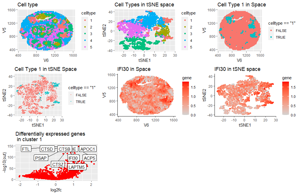
Given the differential gene expression analysis, the cell type equivalent to cluster 1 in the data file is most likely a macrophage. Having identified the overexpressed genes in this cluster (e.g., IFI30,LAPTM5,ACP5,CTSB and CTSZ), ,we search for the names in The Human Protein Atlas under Breast tissue (e.g., https://www.proteinatlas.org/ENSG00000216490-IFI30/tissue+cell+type). Based on the results, the higher correlation was with macrophages. Additionally, there is evidence that each of these genes is upregulated in macrophages in breast cancer tissue. [1,2,3,4,5]

References:

[1] https://www.ncbi.nlm.nih.gov/pmc/articles/PMC8364447/

[2]https://www.ncbi.nlm.nih.gov/pmc/articles/PMC8923652/

[3]https://kns.cnki.net/kcms/detail/detail.aspx?doi=10.16571/j.cnki.1008-8199.2020.07.008

[4]https://www.sciencedirect.com/science/article/pii/S1471490622000941

[5] https://www.ncbi.nlm.nih.gov/pmc/articles/PMC2823914/

################################# Code script:

Based on https://jef.works/genomic-data-visualization-2023/blog/2023/02/17/awang87/

bit.ly/GDV23_visiumBC

data <- read.csv(‘visium_breast_cancer.csv.gz’, row.names=1)

pos <- data[,1:2] gexp <- data[,3:ncol(data)]

normalize

mat <- gexp/rowSums(gexp) mat <- mat*mean(rowSums(gexp)) mat <- log10(mat +1)

TSNE

emb = Rtsne::Rtsne(mat)

Define number of clusters

# install.packages(‘factoextra’)

library(factoextra) library(NbClust) library(cluster) library(ggrepel) ## install.packages(“ggrepel”)

set.seed(0) com <- kmeans(mat, centers=5)

library(ggplot2)

df <- data.frame(pos, emb$Y, celltype = as.factor(com$cluster))

p1 <- ggplot(df, aes(x=V6, y=V5, col=celltype)) + geom_point(size=1.5) + ggtitle(“Cell type”)

p2 <- ggplot(df,aes(x = X1, y = X2 ,col = celltype)) + geom_point(size = 1.5)+labs(x=”tSNE1”,y = “tSNE2”)+ggtitle(“Cell Types in tSNE space”)

p3 <- ggplot(df,aes(x = V6,y = V5,col= celltype == “1”)) + geom_point(size = 1.5) +ggtitle(“Cell Type 1 in Space”)+theme(legend.key.width= unit(.5, ‘cm’)) p4 <- ggplot(df,aes(x = X1, y = X2 ,col = celltype == “1”)) + geom_point(size = .5)+labs(x=”tSNE1”,y = “tSNE2”)+theme(legend.key.width= unit(.5, ‘cm’)) +ggtitle(“Cell Type 1 in tSNE Space”)

library(gridExtra)

cluster.of.interest = names(which(com$cluster == 1)) cluster.other = names(which(com$cluster != 1)) out = sapply(colnames(mat), function(g){ wilcox.test(mat[cluster.of.interest, g],mat[cluster.other, g],alternative=”two.sided”)$p.value })

Choosing a gene:ADAMTS4

gene <- ‘ADAMTS4’

df1 <- data.frame(pos, emb$Y, gene=mat[,gene]) p5 <- ggplot(df1, aes(x = V6, y = V5, col=gene)) + geom_point(size = 1.5) + theme_classic() + scale_color_continuous(low=’lightgrey’, high=’red’) + ggtitle(“ADAMTS4 in Space”) p6 <- ggplot(df1, aes(x = X1, y = X2, col=gene)) + geom_point(size = 1.5) + theme_classic() + scale_color_continuous(low=’lightgrey’, high=’red’) +labs(x=”tSNE1”,y = “tSNE2”)+ggtitle(“ADAMTS4 in tSNE space”)

log2fc <- sapply(colnames(mat), function(g) { a <- mat[cluster.of.interest, g] b <- mat[cluster.other, g] log2(mean(a)/mean(b)) })

volcano plot

df2 = data.frame(out, log2fc) df_subset = df2[names(head(sort(out), n=10)),]

p7 = ggplot(df2, aes(y=-log10(out + 1e-300) , x=log2fc)) + geom_point() +ggtitle(“p-value vs fold change with the top 10 DE gene labels”) + ggrepel::geom_label_repel(data = df_subset, aes(x=log2fc,y=-log10(out+ 1e-300),label = rownames(df_subset)),size = 2.5)

p_genes <- ggplot(df2, aes(y=-log10(out), x=log2fc)) + geom_point(color = “red”) + ggrepel::geom_label_repel(data = df_subset,aes(x=log2fc,y=-log10(out)),max.overlaps = 100,label=rownames(df_subset)) + ggtitle(“Differentially expressed genes \n in cluster 1”)

grid.arrange(p1,p2,p3,p4,p5,p6,p_genes)