Differentially expressed genes and cell-type annotation for cluster 6

Cell-type annotation

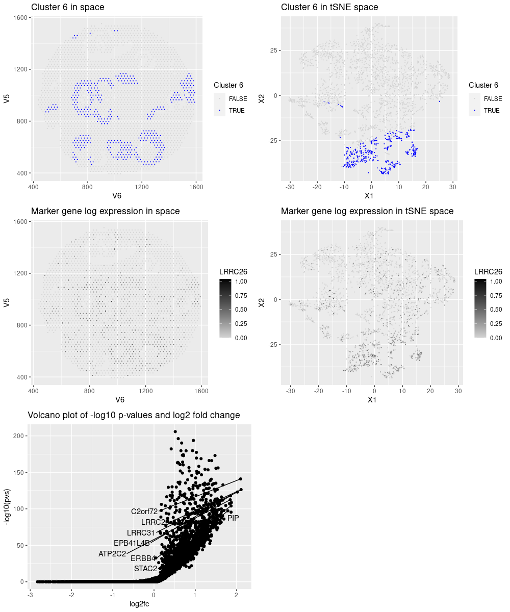
After reading, cleaning and normalizing the data, I performed kmeans clustering and observed that cluster 6 performed an interesting pattern in space. By analysing the most significant genes for that cluster and studying them in The Protein Atlas website (https://www.proteinatlas.org/), I observed that these genes enrich the following groups:

• LRRC26: Cell type enhanced (Intestinal goblet cells, Serous glandular cells, dendritic cells, Prostatic glandular cells, Breast glandular cells)
• C2orf72: Cell type enhanced (Astrocytes, Hepatocytes, Paneth cells, Cholangiocytes, Oligodendrocyte precursor cells, Distal enterocytes)
• LRRC31: Cell type enhanced (Intestinal goblet cells, Enteroendocrine cells, Distal enterocytes, Undifferentiated cells, Paneth cells)
• PAX9: Cell type enhanced (Basal squamous epithelial cells, Squamous epithelial cells, Serous glandular cells, Suprabasal keratinocytes, Basal respiratory cells, Basal keratinocytes)
• ERBB4: Cell type enhanced (Inhibitory neurons, Oligodendrocyte precursor cells, Astrocytes, Oligodendrocytes)
• PIP: Group enriched (Basal prostatic cells, Serous glandular cells)
• INHBB: Group enriched (Granulosa cells, Adipocytes)
• STAC2: Cell type enriched (Muller glia cells)

The genes seem to mark different types. This could be either a characteristic of the genes, or that there are multiple types on the spot. However, Serous glandular cells is the most present group in those genes and it is the cell type chosen to annotate the cluster.

Please share the code you used to reproduce this data visualization.

The code was adapted from HW5.

library(tidyverse)
library(gridExtra)
library(ggrepel)
set.seed(42)

# Preprocessing -----------------------------------------------------------

corner <- function(df){
    df[1:5, 1:5]
}

## load data
data <- read.csv("visium_breast_cancer.csv.gz", row.names = 1)
dim(data)
corner(data)

pos <- data[, 1:2]
gexp <- data[3:ncol(data)]
corner(gexp)

## there are not empty spots or genes
all(rowSums(gexp) > 0)
all(colSums(gexp) > 0)

## plot a histogram of gene counts per spot and log10 gene presence in spots
hist(rowSums(gexp))
hist(log10(colSums(gexp))) # some genes are highly expressed

## normalize cells by total expression and apply log10 +1
totgexp <- rowSums(gexp)
median(totgexp) # 10701, round to 10000
mtx <- gexp/totgexp
mtx <- mtx*10000
mtx <- log10(mtx + 1)



# Reduced dimension and clustering ----------------------------------------

## calculate tsne
emb <- Rtsne::Rtsne(mtx, check = F)

## calculate multiple k means and select k value
kmeans_ss <- lapply(1:15, FUN = function(x){
    com <- kmeans(mtx, centers = x)
    kmeans_vals <- list(wss = com$tot.withinss,
                        bss = com$betweenss,
                        clusters = com$cluster)
    return(kmeans_vals)
})

df_ss <- data.frame(k = 1:15,
                    wss = sapply(kmeans_ss, "[[", 1),
                    bss = sapply(kmeans_ss, "[[", 2))

p_wss <- df_ss %>% ggplot() +
    geom_line(aes(x=k, y=wss))
p_bss <- df_ss %>% ggplot() +
    geom_line(aes(x=k, y=bss))

grid.arrange(p_wss, p_bss)

## based on the graphs, I chose k = 8
com <- kmeans(mtx, centers = 8)
clusters <- com$cluster

## colorblind-friendly palette: http://www.cookbook-r.com/Graphs/Colors_(ggplot2)/
cbbPalette <- c("#000000", "#E69F00", "#56B4E9", "#009E73", "#F0E442", "#0072B2", "#D55E00", "#CC79A7")

## visualize clusters
pos %>%
    mutate(cluster = as.factor(clusters)) %>%
    ggplot() +
    geom_point(aes(V6, V5, color = cluster),
               size = 1.5) +
    scale_color_manual(values = cbbPalette) +
    guides(colour = guide_legend(override.aes = list(size=5)))

## cluster 6 has a nice spatial pattern
plot_clus_pos <- pos %>%
    mutate(cluster = as.factor(clusters)) %>%
    ggplot() +
    geom_point(aes(V6, V5, color = cluster == 6),
               size = .1) +
    scale_color_manual(values = c("lightgray", "blue")) +
    labs(title = "Cluster 6 in space", color = "Cluster 6")
plot_clus_pos

plot_clus_emb <- emb$Y %>%
    data.frame() %>%
    mutate(cluster = as.factor(clusters)) %>%
    ggplot() +
    geom_point(aes(X1, X2, color = cluster == 6),
               size = .1) +
    scale_color_manual(values = c("lightgray", "blue")) +
    labs(title = "Cluster 6 in tSNE space", color = "Cluster 6")
plot_clus_emb


# Differentially expressed genes ------------------------------------------

## select a cluster
selected_cluster <- 6
cluster_of_interest <- names(which(clusters == selected_cluster))
other_clusters <- names(which(clusters != selected_cluster))

## loop through the genes and test each one
genes <- colnames(mtx)
pvs <- sapply(genes, function(g){
    a <- mtx[cluster_of_interest, g]
    b <- mtx[other_clusters, g]
    wilcox.test(a, b, alternative = "greater")$p.val
})

## see marker genes
names(which(pvs < 1e-8))


## calculate a fold change
log2fc <- sapply(genes, function(g){
    a <- mtx[cluster_of_interest, g]
    b <- mtx[other_clusters, g]
    log2(mean(a)/mean(b))
})

sort(log2fc, decreasing = TRUE)[1:15]
# LRRC26  C2orf72   LRRC31     PAX9    ERBB4      PIP EPB41L4B   ATP2C2    INHBB    STAC2
# 2.110030 2.098091 2.020311 1.874843 1.867562 1.867431 1.854935 1.846971 1.828086 1.789061

## According to https://www.proteinatlas.org/
## LRRC26: Cell type enhanced (Intestinal goblet cells, Serous glandular cells, dendritic cells, Prostatic glandular cells, Breast glandular cells)
## C2orf72: Cell type enhanced (Astrocytes, Hepatocytes, Paneth cells, Cholangiocytes, Oligodendrocyte precursor cells, Distal enterocytes)
## LRRC31: Cell type enhanced (Intestinal goblet cells, Enteroendocrine cells, Distal enterocytes, Undifferentiated cells, Paneth cells)
## PAX9: Cell type enhanced (Basal squamous epithelial cells, Squamous epithelial cells, Serous glandular cells, Suprabasal keratinocytes, Basal respiratory cells, Basal keratinocytes)
## ERBB4: Cell type enhanced (Inhibitory neurons, Oligodendrocyte precursor cells, Astrocytes, Oligodendrocytes)
## PIP: Group enriched (Basal prostatic cells, Serous glandular cells)
## INHBB: Group enriched (Granulosa cells, Adipocytes)
## STAC2: Cell type enriched (Muller glia cells)


## half volcano plot
df <- data.frame(pvs, log2fc)
head(df)
plot_deg <- df %>%
    ggplot(aes(log2fc, -log10(pvs))) +
    geom_point() +
    geom_text_repel(aes(label = ifelse(log2fc > 1.78, as.character(rownames(df)), '')),
                    hjust=0, vjust=0) +
    labs(title = "Volcano plot of -log10 p-values and log2 fold change")
plot_deg



head(sort(log2fc, decreasing = T))
g <- names(sort(log2fc, decreasing = T))[1]
g # LRRC26

plot_gene_pos <- pos %>%
    mutate(gene = mtx[,g]) %>%
    ggplot() +
    geom_point(aes(V6, V5, color = gene),
               size = .1) +
    scale_color_gradient(low = "lightgray", high = "black") +
    labs(title = "Marker gene log expression in space", color = g)
plot_gene_pos


plot_gene_emb <- emb$Y %>%
    data.frame() %>%
    mutate(gene = mtx[,g]) %>%
    ggplot() +
    geom_point(aes(X1, X2, color = gene),
               size = .1) +
    scale_color_gradient(low = "lightgray", high = "black") +
    labs(title = "Marker gene log expression in tSNE space", color = g)
plot_gene_emb



## join all plots
grid.arrange(plot_clus_pos, plot_clus_emb,
             plot_gene_pos, plot_gene_emb,
             plot_deg)