Attempts of a cell type identification

A general idea about the exploration
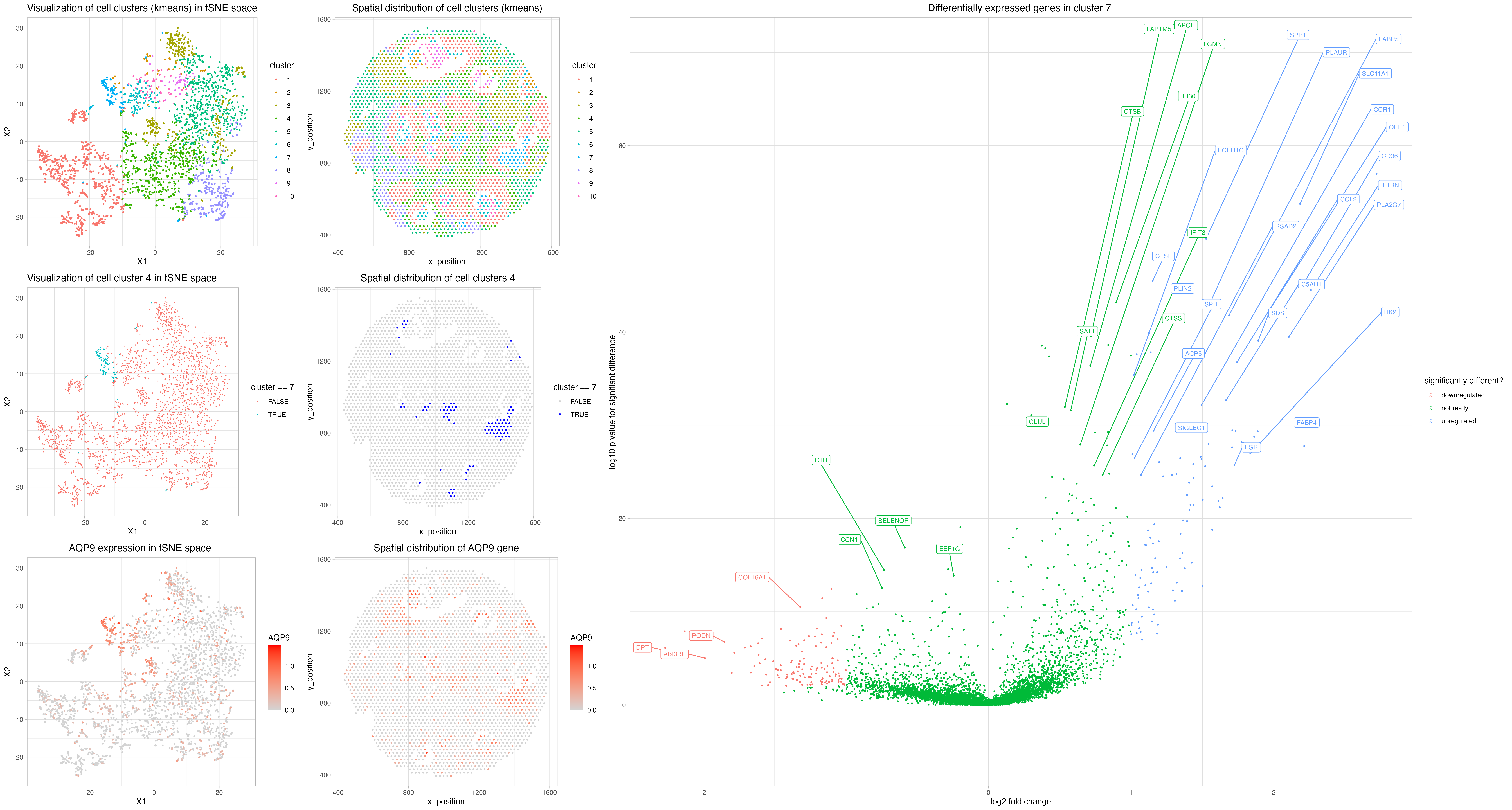
For cluster 7, the most significant genes include
AQP9, IL1RN, FABP4, MMP9, CD36, to a less degree also FCGR3A (CD16a)
https://www.ncbi.nlm.nih.gov/gene/366 https://www.ncbi.nlm.nih.gov/pmc/articles/PMC7699650/ https://www.proteinatlas.org/ENSG00000103569-AQP9 AQP9: most significantly enriched in… liver and appendix? Still, it is related with immune infiltation.(enriched in hepatocytes, monocytes, Kupffer cells, Hofbauer cells, Macrophages)
https://www.wikiwand.com/en/Interleukin-1_receptor_antagonist_protein
IL1RN: “IL1Ra is secreted by various types of cells including immune cells, epithelial cells, and adipocytes, and is a natural inhibitor of the pro-inflammatory effect of IL1β.”
https://www.ncbi.nlm.nih.gov/gene/2167 FABP4: “FABP4 encodes the fatty acid binding protein found in adipocytes. Fatty acid binding proteins are a family of small, highly conserved, cytoplasmic proteins that bind long-chain fatty acids and other hydrophobic ligands. It is thought that FABPs roles include fatty acid uptake, transport, and metabolism. [provided by RefSeq, Jul 2008]”
https://www.ncbi.nlm.nih.gov/pmc/articles/PMC3858212 MMP9: the classic! “MMP-9 is secreted by a wide number of cell types, including neutrophils, macrophages, and fibroblasts.”
https://www.ncbi.nlm.nih.gov/pmc/articles/PMC2811062/ CD36: “CD36 is a membrane glycoprotein present on platelets, mononuclear phagocytes, adipocytes, hepatocytes, myocytes, and some epithelia.”
https://www.proteinatlas.org/ENSG00000203747-FCGR3A FCGR3A: “including lung macrophages, Kupffer cells in liver and non-germinal center cells in lymph node.”
Hence, I assume my cluster of interest to be a mix of adipocytes and immune cells (I am leaning towards macrophages as Kupffer cells ~macrophages). This can be a mix since FABP4 is a really classic adipocyte marker. The result maybe makes sense because the cluster can just happen to be a adipose tissue resident macrophage population.
*Digress: I also tested out cluster 5 but it again semes to be an epithelial cluster. If I have relevant sex information (which I assume to be female), I would assume it to be epithelial ovarian layer.
The most significantly upregulated genes in my cluster 5 (10 kmeans clusters in total) include (to name a few): SFRP4, CCDC80, MXRA8, PODN, DPT
https://www.ncbi.nlm.nih.gov/gene/6424#gene-expression SFRP4: signifcantly enriched in endometrium (ovary) tissues, a bit in urinary bladder. probably epithelial
https://www.ncbi.nlm.nih.gov/gene/151887 CCDC80: significantly expressed in epithelial tissues (maybe maybe), also urinary bladder
https://www.ncbi.nlm.nih.gov/gene/54587#gene-expression MXRA8: significantly expressed in gall bladder, fat, endomerium, ovary, urinary bladder
https://www.ncbi.nlm.nih.gov/gene/1805 DPT: it is most significantly enriched in… fat????
tweaking my hw-3 code :)
Kudos to Gary and Wendy for the color help in the volcano plot!
```{r setup, include=FALSE} knitr::opts_chunk$set(echo = TRUE)
library(ggplot2) library(gridExtra) library(dplyr) library(ggrepel) ## install.packages(“ggrepel”) library(gganimate) library(Rtsne) library(magick)
data <- read.csv(“~/Desktop/GitHub_Repo/genomic-data-visualization-notes/project/visium_breast_cancer.csv”,row.names = 1)
colnames(data)[colnames(data) == ‘V6’] <- ‘x_position’
colnames(data)[colnames(data) == ‘V5’] <- ‘y_position’
1
2
3
4
5
6
7
8
9
10
11
12
13
14
15
16
17
18
19
20
21
22
23
24


``` {r initial processing}

pos <- data[,1:2]
gexp <- data[, 4:ncol(data)]

# screen for ~moderately expressing cells
good.cells <- rownames(gexp)[rowSums(gexp) > 10]
pos <- pos[good.cells,]
gexp <- gexp[good.cells,]

# into a proportion
# note: lose information about gene abundance (absolute counts)
# expand to a scaled value
totgexp <- rowSums(gexp)
mat <- gexp/totgexp
# normalize
mat <- mat*mean(totgexp)
# log transformation
mat <- log10(mat + 1)
# scaling variance
mat.scaled <- scale(mat)
```{r dimensionality reduction + k means clustering} set.seed(0)
emb <- Rtsne::Rtsne(mat.scaled)
pcs <- prcomp(mat.scaled)
top.10.pcs <- data.frame(pcs$x[,1:10])
1
2
3
4
5
6
7
8
9
10
11
12
13
14
15
16


20 iterations is basically running for forever, so keep down to 10 iterations to save my RAM
Maybe I should clean up everything (which I did) but still it is computationally stressing my computer out so I am not running the segment below

Actually the PCs already took over 3 minutes (??? i really should clean my computer)

``` {r explore how many clusters to keep}
# results <- do.call(rbind, lapply(seq_len(10), function(k) {
#   out <- kmeans(mat.scaled, centers=k, iter.max = 10)
#   c(out$tot.withinss, out$betweenss)
# }))
# par(mfrow=c(1,2))
#
# plot(seq_len(10), results[,1], main='tot.withinss')
# plot(seq_len(10), results[,2], main='betweenss')
I here go for a pretty arbitrary cluster number
set.seed(0)
com <- kmeans(mat.scaled, centers=10)

cluster <- com$cluster

tsne.df <- data.frame(pos,
                      emb$Y,
                      cluster = as.factor(cluster))


all.cluster.tSNE <- ggplot(tsne.df,
       aes (x =X1, y = X2, col = cluster)) +
    geom_point(size = 0.5) +
    theme_light() +
    ggtitle("Visualization of cell clusters (kmeans) in tSNE space") +
    theme(plot.title = element_text(hjust = 0.5))

all.cluster.tSNE

all.cluster.space <- ggplot(tsne.df,
       aes (x =x_position, y = y_position, col = cluster)) +
    geom_point(size = 0.5) +
    theme_light() +
    ggtitle("Spatial distribution of cell clusters (kmeans)") +
    theme(plot.title = element_text(hjust = 0.5))

all.cluster.space
```{r loop through the plot to examine interesing cluster} par(mfrow = c(4,dim(com$centers)[1]/4))
loop_plot <- lapply(c(1:dim(com$centers)[1]), function(g) { fig <- ggplot(tsne.df, aes(x = x_position, y = y_position, col = cluster == g)) + geom_point(size = 0.1) + labs(title = paste(“cluster number”, g)) + theme_light() })
loop_plot
1
2
3
4
5
6
7
8
9
10
11
12
13
14
15
16
17
18
19
20
21
22
23
24
25
26
27
28
29
30
31
32
33
34
35
36
37
# cluster 7 seems to internally align each niche (infiltrating???)
Note I tried cluster 4 and it turns out that a lot of genes are only downregulaing without many significantly upregulaing genes, hence I here change to probe cluster 7.

```{r segment the cluster of interest}

cluster7.tSNE <- ggplot(tsne.df, aes(x = X1, y = X2, col = cluster == 7)) +
    geom_point(size = 0.1) +
    ggtitle("Visualization of cell cluster 4 in tSNE space") +
    theme(plot.title = element_text(hjust = 0.5)) +
    theme_light()

cluster7.tSNE

cluster7.space <- ggplot(tsne.df,
       aes (x = x_position, y = y_position, col = cluster == 7)) +
    geom_point(size = 0.5) +
    theme_light() +
    ggtitle("Spatial distribution of cell clusters 4") +
    theme(plot.title = element_text(hjust = 0.5)) +
    scale_color_manual(values=c("lightgrey","blue"))

cluster7.space

cluster.of.interest.df <- data.frame(pos,
                                  emb$Y,
                                  cluster = as.factor(cluster),
                                  target = cluster == 7)

diffgexp <- sapply(colnames(mat), function(g) {
    cluster7 <- names(which(cluster == 7)) # created a variable named cluster well ahead
    ctother <- (names(which(cluster != 4)))
    wilcox.test(mat[cluster7, g],
                mat[ctother,g],
                alternative = "two.sided" )$p.value})

head(sort(diffgexp), n = 20)
```{r log2fc}
log2fc <- sapply(colnames(mat), function(g) { cluster7 <- names(which(cluster == 7)) ctother <- names(which(cluster!= 7)) log2(mean(mat[cluster7,g])/mean(mat[ctother,g])) })
1
2
3
4
5
6
7
8
9
10
11
12
13
14
15
16
17
18
19
20
21
22
23
24
25
26
27
28
29
30
31
32
33
34
35
36
37

Notice here I increased the threshold a bit for significance
```{r log2c -> volcano plot}

log2fc.df <- data.frame(log2fc, pval = diffgexp)

regulated <- apply(log2fc.df, 1, function(g) {
    if (g['pval'] < 0.01 & g['log2fc']> 1) {
    status <- 1 # upregulated
} else if (g['pval'] < 0.01 &g['log2fc']< -1 ) {
    status <- -1 # downregulated
} else {
    status <- 0 # not significant
}
    }
)

log2fc.df <- log2fc.df %>% cbind(regulated)

log2fc.plot <- ggplot(log2fc.df,
       aes(y=-log10(pval),
           x=log2fc,
           col=as.factor(regulated))) +
    geom_point(size = 0.5) +
    ggrepel::geom_label_repel(label=rownames(log2fc.df),
                              max.overlaps = 5,
                              size = 3) +
    scale_color_discrete(name = "significantly different?", labels = c("downregulated", "not really", "upregulated")) +
    ggtitle("Differentially expressed genes in cluster 7 ") +
    xlab("log2 fold change") +
    ylab("log10 p value for signifiant difference") +
    ylim(-5,70) +
    theme_light() +
    theme(plot.title = element_text(hjust = 0.5))


log2fc.plot
The most significantly upregulated genes include (to name a few) AQP9, IL1RN, FABP4, MMP9, CD36, CTSL, PLN2, OLR1, SPP1, FCGR3A, CCL2
Based on the graph, AQP9 seems like an interesting gene
```{r visualize AQP9}
tsne.df$AQP9 <- mat$AQP9 AQP9.tsne <- ggplot(tsne.df, aes(x = X1, y = X2, col = AQP9)) + geom_point(size = 0.5) + scale_color_gradient(low = ‘lightgrey’,high = ‘red’) + ggtitle(“AQP9 expression in tSNE space “) + theme_light() + theme(plot.title = element_text(hjust = 0.5))
AQP9.tsne
AQP9.space <- ggplot(tsne.df, aes (x =x_position, y = y_position, col = AQP9)) + geom_point(size = 0.5) + scale_color_gradient(low = ‘lightgrey’,high = ‘red’) + theme_light() + ggtitle(“Spatial distribution of AQP9 gene”) + theme(plot.title = element_text(hjust = 0.5))
AQP9.space
1
2
3
4
5
6
7
8
9
10
11
12
13
14
15
16
17
18
19


``` {r plot}

final.plot <- arrangeGrob(all.cluster.tSNE,all.cluster.space,
                           cluster7.tSNE,cluster7.space,
                           AQP9.tsne,AQP9.space,
                           log2fc.plot,
                          layout_matrix = rbind(c(1,2,7,7,7),
                                                c(3,4,7,7,7),
                                                c(5,6,7,7,7)
                                               ))

ggsave(file = "final.png",
       final.plot,
       width = 28,
       height = 15)
