Identification of the Breast Cancer Cells

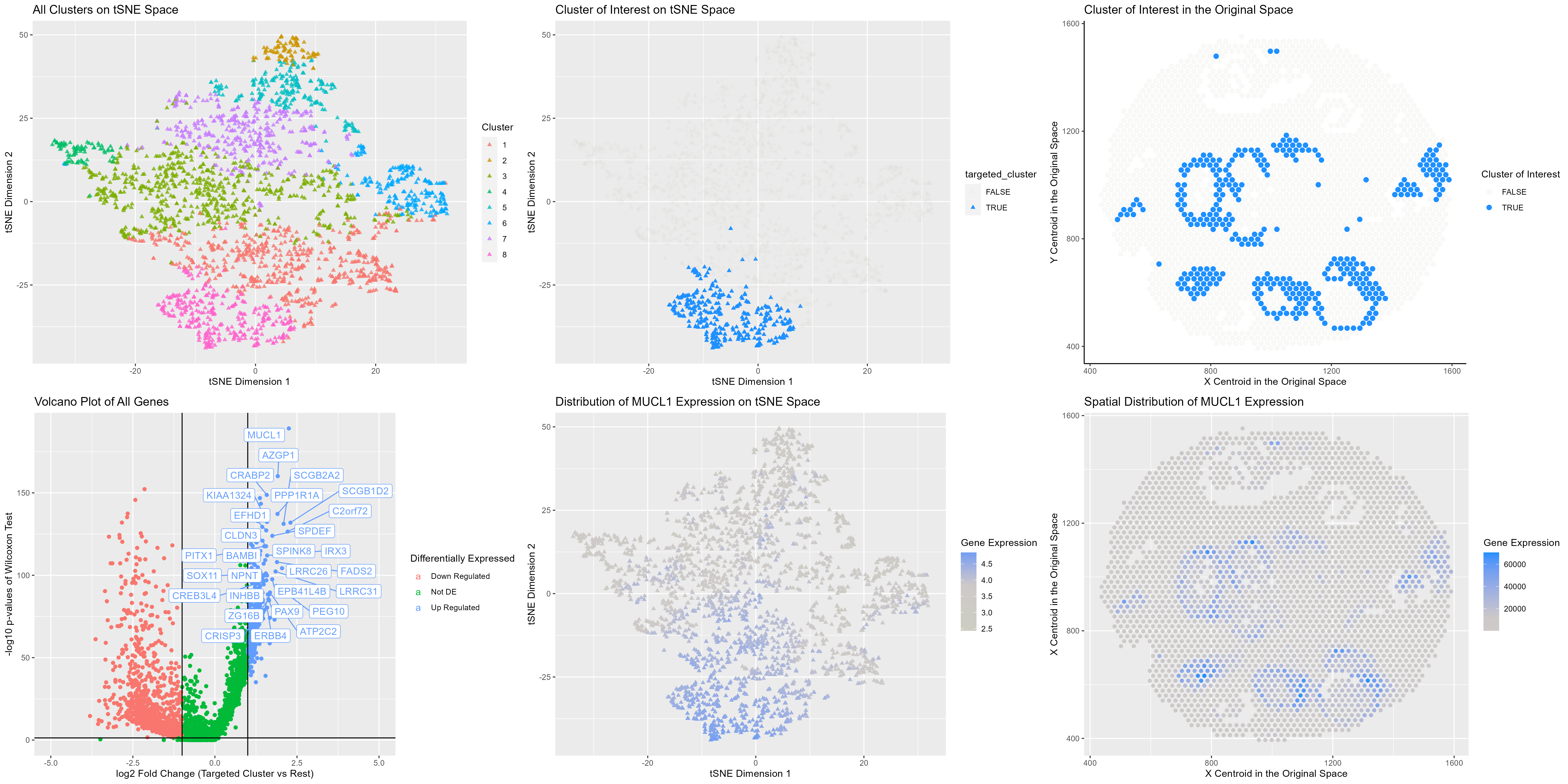
The visualization presented above comprises six panels, all of which provide evidence to support the hypothesis that cluster 8 corresponds to breast cancer cells. The top row panels are referred to as A, B, and C, while the bottom row panels are labeled D, E, and F.

Kmeans clustering were done on first 150 principal components of the normalized (but not log-transformed) data. Seven clusters were identified (panel A). The analysis focuses on cluster 8 (panel B), which appear to form semi circular or blobular pattern (panel C). After splitting the dataset into two groups, cluster 8 and the rest, I performed differential expression analysis. Many genes showed strong up- and down-regulation patterns (panel D). Many of genes, such as MUCL1, CREB3L4, And ERRB4 have significantly high expression in breast tissues, according to Human Protein Atlas (1). However, many literatures have also reported the overexpression of these proteins in breast cancer cells (2-5); thus, I believe the cluster I identified corresponds to breast cancer cells. Panel E and F shows the specificity of MUCL2 expression, mainly restricted to cluster 8.

1. https://www.proteinatlas.org/
2. https://link.springer.com/article/10.1007/s10911-008-9079-3
3. https://pubmed.ncbi.nlm.nih.gov/25590338/
4. https://link.springer.com/article/10.1007/s10911-020-09443-6
5. https://www.nature.com/articles/onc2015487

Code took inspiration from https://biocorecrg.github.io/CRG_RIntroduction/volcano-plots.html

Much of the code/analysis were adopted from my previous homework assignment.

Code

library(ggplot2)
library(irlba)
library(Rtsne)
library(gridExtra)
library(ggrepel)

# bit.ly/GDV23_visiumBC
data <- read.csv('visium_breast_cancer.csv.gz', row.names=1)
posn <- data[,1:2]
gexp <- data[,3:ncol(data)]
rownames(posn) <- rownames(gexp) <- data$X

## Normalization
totgexp <- rowSums(gexp)
gexp <- gexp/totgexp
gexp <- gexp*1e6

# Dimensionality Reduction
pcs <- prcomp_irlba(gexp, 150)
plot(pcs$sdev[1:150], type="l")

# For reproducibility.
set.seed(42)
emb1 <- Rtsne(pcs$x)

## K-means
set.seed(42)
com <- kmeans(pcs$x, centers=8, iter.max=100)
clusters <- as.factor(com$cluster) ## for categorical

# Plot cells on a tSNE embedded space, color cells by cluster assignment
all_cluster_tsne <- data.frame(emb1$Y, clus=clusters)
p3 <- ggplot(all_cluster_tsne, 
             aes(x=X1, y=X2, col=clus)) +
  geom_point(alpha=0.8, shape=17) +
  labs(x="tSNE Dimension 1", 
       y="tSNE Dimension 2",       
       title="All Clusters on tSNE Space", 
       color="Cluster")

## Focus on cluster #1
cluster_of_interest <- 8
targeted_cluster    <- clusters == cluster_of_interest

targeted_cluster_vs_rest_tsne <- data.frame(emb1$Y, clus=clusters)
p4 <- ggplot(targeted_cluster_vs_rest_tsne, 
             aes(x=X1, 
                 y=X2, 
                 col=targeted_cluster, 
                 alpha=targeted_cluster)) +
  geom_point(shape=17) +
  labs(x="tSNE Dimension 1", 
       y="tSNE Dimension 2",        
       title="Cluster of Interest on tSNE Space") + 
  scale_color_manual(values=c("#CDCDC1", "#1E90FF")) 

## Visualize cluster of interest in original space
data_clus <- cbind(posn, gexp, targeted_cluster)
p1 <- ggplot(data=data_clus, 
             aes(x=V6, 
                 y=V5)) + 
  geom_point(aes(color=targeted_cluster, alpha=targeted_cluster), 
             shape =19,
             stroke=1) + 
  scale_color_manual(values=c("#CDCDC1", "#1E90FF")) + 
  theme_classic() + 
  labs(x="X Centroid in the Original Space", 
       y="Y Centroid in the Original Space",       
       title="Cluster of Interest in the Original Space", 
       color="Cluster of Interest", alpha="Cluster of Interest")

## Subset out cluster of interest vs others
target.cells <- which(com$cluster == cluster_of_interest)
others.cells <- which(com$cluster != cluster_of_interest)

## Test for differential expression
## Compute p-vals and log2 Fold Change
genes <- colnames(gexp)
pvs <- sapply(genes, function(g) {
  a <- gexp[target.cells, g]
  b <- gexp[others.cells, g]
  wilcox.test(a,b,alternative="two.sided")$p.val
})
log2fc <- sapply(genes, function(g) {
  a <- gexp[target.cells, g]
  b <- gexp[others.cells, g]
  log2(mean(a)/mean(b))
})

## Categorize points into classes, fix points with loss of precision
volcano_df <- data.frame(pvs, log2fc)
volcano_df$deg_status <- "Not DE"
volcano_df$deg_status[volcano_df$log2fc > 1  & volcano_df$pvs < 0.05] <- "Up Regulated"
volcano_df$deg_status[volcano_df$log2fc < -1 & volcano_df$pvs < 0.05] <- "Down Regulated"
volcano_df$display_name <- NA
volcano_df$display_name[volcano_df$log2fc > 1.5  & -log10(volcano_df$pvs) > 80] <- 
  rownames(volcano_df)[volcano_df$log2fc > 1.5  & -log10(volcano_df$pvs) > 80]
volcano_df$pvs[volcano_df$pvs == 0] <- 1e-300

## Inspired by https://biocorecrg.github.io/CRG_RIntroduction/volcano-plots.html
## Volcano Plot
p2 <- ggplot(volcano_df, 
             aes(y=-log10(pvs), 
                 x=log2fc, 
                 color=deg_status)) + 
  geom_point() +  
  geom_vline(xintercept=c(-1, 1)    , col="black") +
  geom_hline(yintercept=-log10(0.05), col="black") + 
  ggrepel::geom_label_repel(label=volcano_df$display_name, max.overlaps=100) + 
  xlim(-5, 5) + 
  #ylim(-10, 350) +
  labs(x="log2 Fold Change (Targeted Cluster vs Rest)", 
       y="-log10 p-values of Wilcoxon Test", 
       title="Volcano Plot of All Genes", 
       color="Differentially Expressed")

# Plot cells on a tSNE embedded space, color cells by MUCL1
MUCL1_tsne <- data.frame(emb1$Y, gene_expr=log10(gexp["MUCL1"]+1), targeted_cluster=targeted_cluster)
colnames(MUCL1_tsne) <- c("X1", "X2", "gene_expr", "targeted_cluster")
p5 <- ggplot(MUCL1_tsne, aes(x=X1, y=X2, col=gene_expr)) +
  geom_point(shape=17) +
  scale_color_gradient2(low="#CDCDC1", high="#1E90FF", mid="#CDC9C9", midpoint=colMeans(log10(gexp["MUCL1"]+1))) +
  labs(x="tSNE Dimension 1", 
       y="tSNE Dimension 2",       
       title="Distribution of MUCL1 Expression on tSNE Space", 
       color="Gene Expression", 
       alpha="Targeted Cluster")

# Plot cells on the original space, color cells by MUCL1
MUCL1_original <- data.frame(posn, gene_expr=gexp["MUCL1"], targeted_cluster=targeted_cluster)
colnames(MUCL1_original) <- c("X1", "X2", "gene_expr", "targeted_cluster")
p8 <- ggplot(MUCL1_original, aes(x=X1, y=X2, col=gene_expr)) +
  geom_point() +
  scale_color_gradient2(low="#CDCDC1", high="#1E90FF", mid="#CDC9C9", midpoint=colMeans(gexp["MUCL1"])) +
  labs(x="X Centroid in the Original Space", 
       y="X Centroid in the Original Space", 
       title="Spatial Distribution of MUCL1 Expression", 
       color="Gene Expression", 
       alpha="Targeted Cluster")

g <- arrangeGrob(p3,p4,p1,p2,p5,p8,
                 layout_matrix=rbind(c(1,2,3),c(4,5,6))) #generates g
ggsave(file="hw6_yyang117.png",
       g,
       height=12,
       width=24,
) #saves g