Cells Clustered By Protein Levels

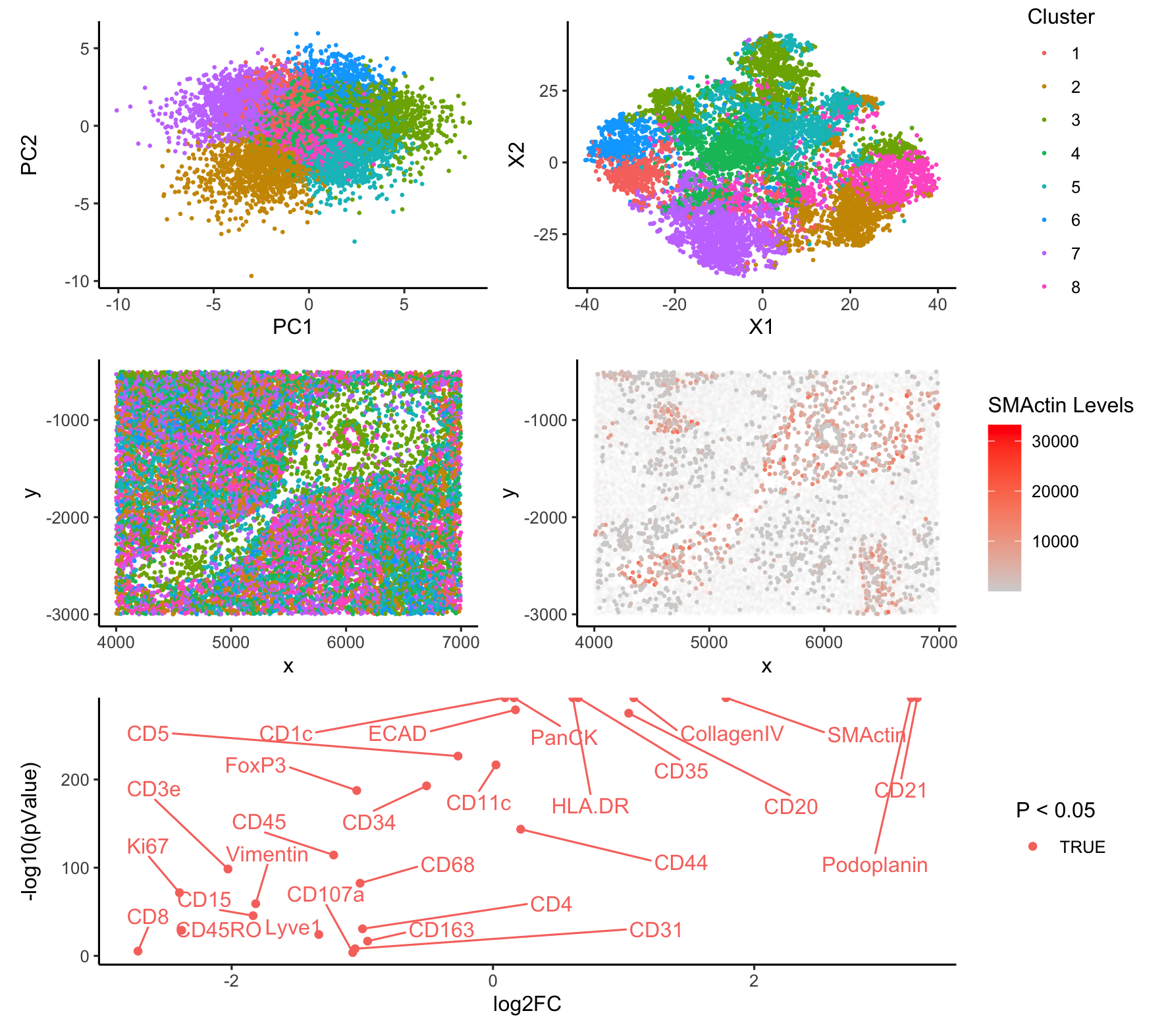
I suspect that cluster 3 represents follciular dendritic cells (FDCs). A number of proteins are significantly upregulated in cluster 3, including SMActin, Podoplanin, and CD21/CD35. SMActin is found in a variety of cell types and has previously been used as a marker for endothelial cells (Dayao et al, 2022). However, this is not particularly consistent with the other top hits.

Previous research indicates that CD21 and CD35 are expressed in pairs in FDCs (Wang et al, 2011). FDCs are known to occur in the spleen and have also been shown to express SMActin (Muñoz-Fernández, 2014). Likewise, Yu, et al 2007 demonstrates that Podoplanin, another of the highly upregulated genes, is an FDC marker, albeit in the case of tumorogenesis.

Code:

`library(ggplot2)
library(tidyverse)
library(Rtsne)
library(patchwork)
library(ggrepel)

data <- read.csv('~/genomic_data_viz/codex_spleen_subset.csv.gz',
                 row.names = 1)

# Initial Spatial Plotting
ggplot(data = data, aes(x=x, y=y)) +
  geom_point()

# Subset data into spatial info and gene expression
pos <- data[, 1:3]
gexp <- data[, 4:ncol(data)]

### QC
# Plotting protein abundance per cell
hist(rowSums(gexp))

ggplot(data = data, aes(x=x, y=y, col = rowSums(gexp))) +
  scale_color_gradient(low='lightgrey', high='red') +
  geom_point()

# Lots of variation in protein abundance, but with no obvious spatial pattern 

# Plotting 
hist(colSums(gexp), breaks = 100)
min(colSums(gexp))

# This has some pretty extreme outliers

# Normalizing
mat <- gexp / rowSums(gexp) * median(rowSums(gexp))
mat <- log10(mat + 1)
mat <- scale(mat)


# Checking that this worked correctly 
hist(rowSums(mat))
hist(colSums(mat))


# Clustering 
# Finding optimal number of clusters
within_ss_list <- c()
max_clust = 25
for (i in 1:max_clust){
  set.seed(0)
  k <- kmeans(mat, centers=i)
  within_ss_list <- c(within_ss_list, k$tot.withinss)	
}

pltDF <- data.frame(k = 1:max_clust, withinSS <- within_ss_list)
ggplot(pltDF, aes(x = k, y = within_ss_list)) + 
  geom_point() + 
  theme_classic() + 
  scale_x_continuous(breaks=seq(1,max_clust,1),labels=seq(1,max_clust,1))

# Clustering fr 
set.seed(0)
pc <- prcomp(mat)
set.seed(0)
n_centers = 8
set.seed(0)
k <- kmeans(mat, centers = n_centers)

set.seed(0)
emb <- Rtsne(mat)

# Plotting 

pca_plot <- ggplot(data.frame(pc$x), aes(x=PC1, y=PC2, color = factor(k$cluster))) +
  geom_point(size=0.4) +
  theme_classic() + 
  theme(legend.position="none")

tsne_plot <- ggplot(data.frame(emb$Y), aes(x=X1, y=X2, color = factor(k$cluster))) +
  geom_point(size=0.4) +
  labs(colour="Cluster") + 
  theme_classic() 

spatial_cluster_plot <- ggplot(pos, aes(x=x, y=y, color = factor(k$cluster))) +
  geom_point(size=0.4) +
  theme_classic() + 
  theme(legend.position="none")


for (i in seq(1, n_centers)){
  print(ggplot(pos, aes(x=x, y=y, color = (factor(k$cluster)==i))) +
    geom_point() + 
    theme_classic() +
    ggtitle(i) +
    theme(axis.title.x = element_blank(),
          legend.position="none")
  )
}

cluster.cells <-  names(which(k$cluster == 3))
other.cells <- names(which(k$cluster != 3))

# First, comparing clusters 1+8 against all else
diff<- sapply(colnames(mat), function(g){
  wilcox.test(mat[cluster.cells, g],
              mat[other.cells, g],
              alternative = 'two.sided')$p.value
  
})

head(sort(diff), n = 30)
diff_names <- names(diff[diff < 0.05/length(diff)])

ggplot(pos, aes(x=x, y=y, color = factor(k$cluster)==3)) +
  geom_point() +
  theme_classic()

smactin <- ggplot(pos, aes(x=x, y=y, color = data.frame(gexp)$SMActin, alpha = factor(k$cluster))) +
  geom_point(size=0.4) + 
  labs(color='SMActin Levels') +
  scale_alpha_manual(values = c(rep(0.05, 2), 1, rep(0.05,5)), guide = 'none') +
  scale_color_gradient(low = 'lightgrey', high = 'red') +
  theme_classic()


fc <- sapply(colnames(gexp), function(g){
  log2(mean(gexp[cluster.cells, g])/mean(gexp[other.cells, g]))
})

df_volcano <- data.frame(log2FC = fc, pValue = diff, comparison = "Group 4 vs All Others")

df_volcano$gname <- rownames(df_volcano)

volcano_plot <- ggplot(df_volcano, aes(x = log2FC, y = -log10(pValue), color = pValue < (0.05/ncol(mat)))) +
  geom_point() + 
  theme_classic() + 
  labs(color='P < 0.05') +
  geom_text_repel(data = df_volcano %>% 
                    mutate(label = ifelse(gname %in% diff_names,
                                          gname, "")),
                  aes(label = label), 
                  box.padding = 1,
                  show.legend = FALSE, 
                  max.overlaps = Inf)
    
(pca_plot | tsne_plot )/ (spatial_cluster_plot |smactin) / volcano_plot

References Dayao, M.T., Brusko, M., Wasserfall, C. et al. Membrane marker selection for segmenting single cell spatial proteomics data. Nat Commun 13, 1999 (2022).

Muñoz-Fernández R, Prados A, Tirado-González I, Martín F, Abadía AC, Olivares EG. Contractile activity of human follicular dendritic cells. Immunol Cell Biol. 2014 Nov;92(10):851-9. doi: 10.1038/icb.2014.61. Epub 2014 Aug 26. PMID: 25155466.

Xiaoming Wang, Bryan Cho, Kazuhiro Suzuki, Ying Xu, Jesse A. Green, Jinping An, Jason G. Cyster; Follicular dendritic cells help establish follicle identity and promote B cell retention in germinal centers. J Exp Med 21 November 2011; 208 (12): 2497–2510. doi: https://doi.org/10.1084/jem.20111449

Yu H, Gibson JA, Pinkus GS, Hornick JL. Podoplanin (D2-40) is a novel marker for follicular dendritic cell tumors. Am J Clin Pathol. 2007 Nov;128(5):776-82. doi: 10.1309/7P8U659JBJCV6EEU. PMID: 17951199.