Cell Type Exploration of CODEX Spleen Data Set

Description:
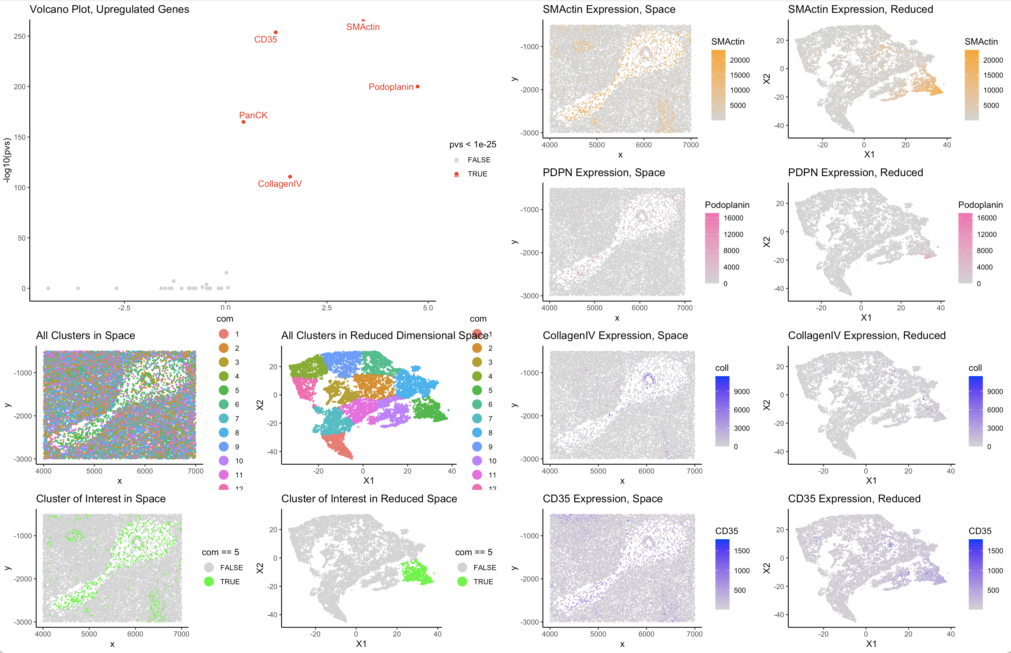
Based on the interesting spatial structure, I chose cluster 5. Cluster 5 was differentially upregulated in the proteins smooth muscle actin, podoplanin, collagenIV, and CD35. Smooth muscle actin, podoplanin, and collagenIV are all structural proteins when in conjunction point to the cell type represented by this cluster being reticular fibroblast cells. In the spleen reticular fibroblast cells are responsible for maintain the extracellular connective structure throughout the cell. It makes sense, therefore that collagen and smooth muscle fibers are highly expressed as these are important components of the ECM. The connective structures created by the excretion of these proteins create a network which immune cells can travel on to get to the place they are needed for further maturation/specification in the spleen. Podoplanin contributes to this network by managing contractility of reticular fibroblast cells. The presence of CD35 which are expressed in lymphocytes are likely also upregulated in the spatial region of the reticular cells as they probably travelling on the network created by the reticular cells.The expression of CD35 is also nonspecific to this cluster, so recognizing the specificity of the expression of the other highly regulated proteins, I conclude that this cluster is picking up on reticular fibroblast spleen cells.
Sources: https://academic.oup.com/intimm/article/25/1/25/2357292 https://www.cell.com/trends/immunology/fulltext/S1471-4906%2821%2900120-4 https://www.ncbi.nlm.nih.gov/pmc/articles/PMC4270928/ https://en.wikipedia.org/wiki/Reticular_cell#:~:text=Reticular%20cells%20are%20found%20in,mesenchymal%2C%20and%20fibroblastic%20reticular%20cells. https://www.biologyonline.com/dictionary/reticular-connective-tissue#:~:text=The%20reticular%20fibers%20are%20made,lymph%20nodes%2C%20and%20bone%20marrow.
Code:
1
2
3
4
5
6
7
8
9
10
11
12
13
14
15
16
17
18
19
20
21
22
23
24
25
26
27
28
29
30
31
32
33
34
35
36
37
38
39
40
41
42
43
44
45
46
47
48
49
50
51
52
53
54
55
56
57
58
59
60
61
62
63
64
65
66
67
68
69
70
71
72
73
74
75
76
77
78
79
80
81
82
83
84
85
86
87
88
89
90
91
92
93
94
95
96
97
98
99
100
101
102
103
104
105
106
107
108
109
110
111
112
113
114
115
116
117
118
119
120
121
122
123
124
125
126
127
128
129
130
131
132
133
134
135
library(ggplot2)
library(gridExtra)

#all code from in class/previous homeworks unless otherwise stated
data <- read.csv('~/Desktop/codex_spleen_subset (1).csv.gz', row.names = 1)

dim(data)

head(data)
pos <- data[,1:2]
area <- data[,3]
exp <- data[,4:ncol(data)]

#QC/normalize by cell
mat <- exp/rowSums(exp)
mat <- mat*mean(rowSums(exp))


pcs <- prcomp(mat)
pcs <- pcs$x[,1:10]

emb <- Rtsne::Rtsne(pcs, perplexity = 100, check = FALSE)

#decide on the number of clusters
ks <- 1:20
out <- do.call(rbind, lapply(ks, function(k){
  com <- kmeans(emb$Y, centers=k)
  c(within = com$tot.withinss, between = com$betweenss)
}))

plot(ks, out[,1], type="l")
plot(ks, out[,2], type="l")

com <- kmeans(emb$Y, centers=12)

df <- data.frame(pos, emb$Y, com=as.factor(com$cluster))
# source: legend size: https://www.geeksforgeeks.org/control-size-of-ggplot2-legend-items-in-r/
p1 <- ggplot(df, aes(x = x, y = y, col=com)) + geom_point(size = 0.4) +
  theme_classic() + guides(color = guide_legend(override.aes = list(size = 5))) +
  ggtitle('All Clusters in Space')

p2 <- ggplot(df, aes(x = X1, y = X2, col=com)) + geom_point(size = 0.4) +
  theme_classic() + guides(color = guide_legend(override.aes = list(size = 5))) +
  ggtitle('All Clusters in Reduced Dimensional Space')

#source for true/false coloring: https://stackoverflow.com/questions/15417220/ggplots-conditional-colour-scale
p3 <- ggplot(df, aes(x = x, y = y, col= com == 5)) + geom_point(size = 0.2) +
  theme_classic() + guides(color = guide_legend(override.aes = list(size = 5))) +
  scale_color_manual(values=c("FALSE"="lightgrey","TRUE"="green")) +
  ggtitle('Cluster of Interest in Space')

p4 <- ggplot(df, aes(x = X1, y = X2, col= com == 5)) + geom_point(size = 0.2) +
  theme_classic() + guides(color = guide_legend(override.aes = list(size = 5))) +
  scale_color_manual(values=c("FALSE"="lightgrey","TRUE"="green")) +
  ggtitle('Cluster of Interest in Reduced Space')

grid.arrange(p1,p2, p3, p4, ncol = 2)


gene_names <- colnames(exp)

#source: Todd's "Cell Exploration of Charmander Data Set" https://jef.works/genomic-data-visualization-2023/blog/2023/02/17/thartm10/
cluster.cells <- which(com$cluster == 5)
other.cells <- which(com$cluster != 5)

pvs <- sapply(gene_names, function(g) {
  a <- exp[cluster.cells, g]
  b <- exp[other.cells, g]
  wilcox.test(a,b,alternative="greater")$p.val
})

log2fc <- sapply(gene_names, function(g) {
  a <- exp[cluster.cells, g]
  b <- exp[other.cells, g]
  log2(mean(a)/mean(b))
})
upreg <- pvs[pvs < 1e-25]
df2 <- data.frame(pvs, log2fc)
upreg_gene_names = names(which(pvs < 1e-25))


p_volcano<- ggplot(df2, aes(y=-log10(pvs), x=log2fc, col = pvs < 1e-25)) + geom_point() +
  scale_color_manual(values = c('lightgrey','red')) +
  ggrepel::geom_text_repel(data = df2[pvs < 1e-25,], label = upreg_gene_names) +
  ggtitle('Volcano Plot, Upregulated Genes') + theme_classic()
p_volcano

df <- data.frame(pos, emb$Y, com=as.factor(com$cluster), SMActin = mat[, 'SMActin'], Podoplanin = mat[,'Podoplanin'], coll = mat[,'CollagenIV'], CD35 = mat[,'CD35'],
                 CD4 = mat[,'CD4'], CD3e = mat[,'CD3e'])
pSMActin_tsne <- ggplot(df, aes(x = X1, y = X2, col= SMActin)) + geom_point(size = 0.1) +
  theme_classic()  + scale_color_continuous(low = 'lightgrey', high= 'orange') +
  ggtitle('SMActin Expression, Reduced')


pSMActin_space <- ggplot(df, aes(x = x, y = y, col = SMActin)) + geom_point(size = .1) +
  scale_color_continuous(low = "lightgrey", high = "orange") +
  ggtitle('SMActin Expression, Space') + theme_classic()


pPDPN_tsne <- ggplot(df, aes(x = X1, y = X2, col= Podoplanin)) + geom_point(size = 0.1) +
  theme_classic()  + scale_color_continuous(low = 'lightgrey', high= 'hotpink') +
  ggtitle('PDPN Expression, Reduced') + theme_classic()


pPDPN_space <- ggplot(df, aes(x = x, y = y, col = Podoplanin)) + geom_point(size = .1) +
  scale_color_continuous(low = "lightgrey", high = "hotpink") +
  ggtitle('PDPN Expression, Space') + theme_classic()

pcoll_tsne <- ggplot(df, aes(x = X1, y = X2, col= coll)) + geom_point(size = 0.1) +
  theme_classic()  + scale_color_continuous(low = 'lightgrey', high= 'blue') +
  ggtitle('CollagenIV Expression, Reduced') + theme_classic()


pcoll_space <- ggplot(df, aes(x = x, y = y, col = coll)) + geom_point(size = .1) +
  scale_color_continuous(low = "lightgrey", high = "blue") +
  ggtitle('CollagenIV Expression, Space') + theme_classic()

pCD35_tsne <- ggplot(df, aes(x = X1, y = X2, col= CD35)) + geom_point(size = 0.1) +
  theme_classic()  + scale_color_continuous(low = 'lightgrey', high= 'blue') +
  ggtitle('CD35 Expression, Reduced') + theme_classic()


pCD35_space <- ggplot(df, aes(x = x, y = y, col = CD35)) + geom_point(size = .1) +
  scale_color_continuous(low = "lightgrey", high = "blue") +
  ggtitle('CD35 Expression, Space') + theme_classic()

#source: Gohta's "Running tSNE analysis on genes or PCs"  https://jef.works/genomic-data-visualization-2023/blog/2023/02/06/gaihara1/
lay <- rbind(c(1,1,6,7),
             c(1,1,8,9),
             c(2,3,10,11),
             c(4,5,12,13))


grid.arrange(p_volcano, p1, p2, p3, p4, pSMActin_space,pSMActin_tsne,
             pPDPN_space, pPDPN_tsne, pcoll_space, pcoll_tsne,pCD35_space, pCD35_tsne,layout_matrix = lay)