Determination of Cell Cluster 5 as Natural Killer Cells

What cell type is the cluster you picked and what went in to your determination?
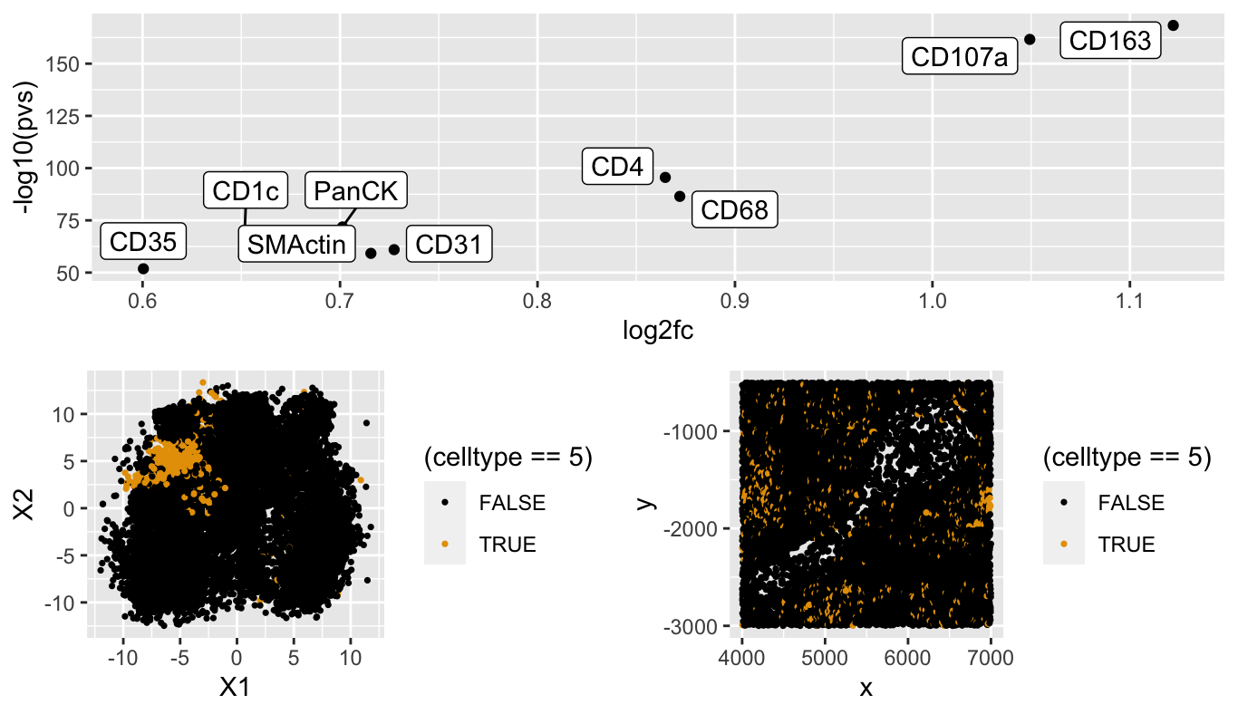
I have identified cell cluster 5 as being Natural Killer cells due the differential expression analysis that I performed that showed that CD163 and CD107a were both significantly upregulated in the cluster. These two proteins are identified as being markers for immune cells and specfiically as markers of natural killer cells. Additionally, when looking at the spatial distribution of cells in cluster 5, they appear to grouped in clumps but still pretty spread out which matches the descpriton of Natural Killer cells.
https://pubmed.ncbi.nlm.nih.gov/15604012/ https://www.ncbi.nlm.nih.gov/gene/9332
library(Rtsne)
library(tidyverse)
library(ggokabeito)
library(gganimate)
library(gifski)
library(ggrepel)
library(gridExtra)
library(rcartocolor)
library(grid)
library(ggplotify)

##Most code adapted from Prof. Fan "code-02-13-2023" code unless otherwise noted
data <- read.csv('Downloads/codex_spleen_subset.csv.gz')

##Capture gene expression

pos <- data[,2:3]
gexp <- data[,5:ncol(data)]

##Normalize
good.cells <-rownames(gexp)[rowSums(gexp) > 10]
pos <- pos[good.cells,]
gexp <- gexp[good.cells,]

totgexp <- rowSums(gexp)
mat <- gexp/totgexp
# normalize
mat <- mat*median(totgexp)
# log transformation
mat <- log10(mat + 1)
# scaling variance
mat.scaled <- scale(mat)

colorblind_palette <- c("#000000","#E69F00","#56B4E9","#009E73","#F0E442",
                                 "#0072B2","#D55E00","#CC79A7","#999999","#88CCEE", "#CC6677", "#DDCC77", "#117733", "#332288", "#AA4499",
                                 "#44AA99", "#999933", "#882255", "#661100", "#6699CC", "#888888")


#find principal component number that makes sense (taken from class)
pcs <- prcomp(mat.scaled)
par(mfrow=c(1,1))
plot(1:50,pcs$sdev[1:50],type='l')

#Using above graph, used only six principal components
set.seed(8)
pcsIm <- pcs$x[,1:22]
emb <- Rtsne::Rtsne(pcsIm,perplexity=500)

#Taken from Prof. Fan/I think Ryan in class on how to decide how many clusters to pick (10)
results <- do.call(rbind, lapply(seq_len(30), function(k) {
  out <- kmeans(pcsIm,centers=k, iter.max=50)
  c(out$tot.withinss,out$betweenss)
}))
plot(seq_len(30),results[,1], main='tot.withinss',type='b', xlab='# Centers')
plot(seq_len(30),results[,2], main='tot.betweenss',type='b', xlab='# Centers')

com <- kmeans(pcsIm, centers=21)


df <- data.frame(pos, emb$Y, celltype=as.factor(com$cluster))
head(df)
p1 <- ggplot(df, aes(x = X1, y = X2, col=(celltype==5))) + geom_point(size = 0.6) +
  scale_color_manual(values=colorblind_palette)
p2 <- ggplot(df, aes(x = x, y = y, col=(celltype==5))) +
  geom_point(size = 0.6) + scale_color_manual(values=colorblind_palette)

grid.arrange(p1,p2)

## pick a cluster
cluster.of.interest <- names(which(com$cluster == 5))
cluster.other <- names(which(com$cluster != 5))

genes <- colnames(mat.scaled)
pvs <- sapply(genes, function(g) {
  a <- mat.scaled[cluster.of.interest, g]
  b <- mat.scaled[cluster.other, g]
  wilcox.test(a,b,alternative="two.sided")$p.val
})

log2fc <- sapply(genes, function(g) {
  a <- mat.scaled[cluster.of.interest, g]+1
  b <- mat.scaled[cluster.other, g]+1
  log2(mean(a)/mean(b))
})

df2 <- data.frame(pvs, log2fc)
df2 = df2[df2$pvs < 1e-50 & df2$log2fc > 0.5,]
#df2 = df2[df2$pvs < 1e-150 & df2$log2fc > 1.5,]

p3 <- ggplot(df2, aes(y=-log10(pvs), x=log2fc)) + geom_point() +
  ggrepel::geom_label_repel(label=rownames(df2))

df3 <- data.frame(pos, emb$Y, gexp)
p4 <- ggplot(df3, aes(x = X1, y = X2, col=CD56)) + geom_point(size = 0.8) +
  theme_classic()
p5 <- ggplot(df3, aes(x = x, y = y, col=CD56)) +
  geom_point(size = 0.8) + theme_classic()

grid.arrange(p3,grid.arrange(ncol=2,p1,p2))