Determining the relationship between gene expression and physical spaces

1. Write a description explaining why you believe your data visualization is effective using vocabulary terms from Lesson 1.
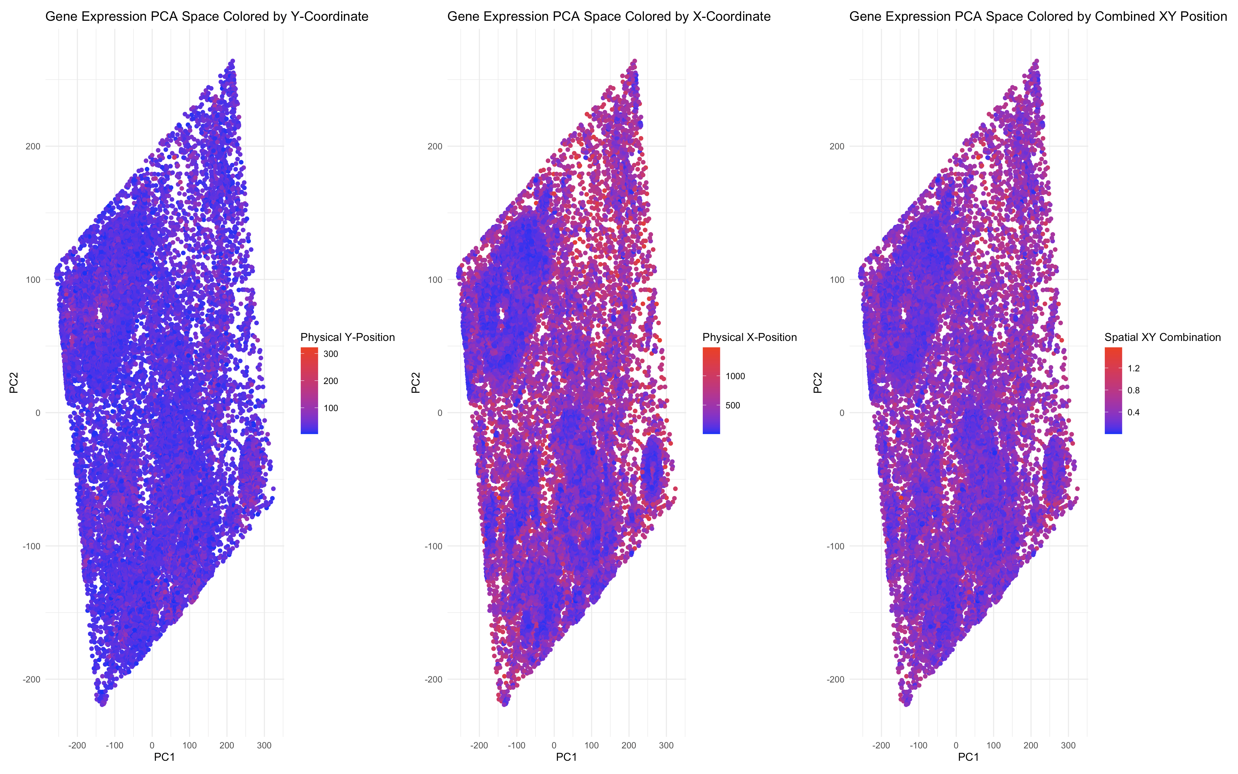
This visualization explores how gene expression patterns relate to spatial organization by projecting high-dimensional gene expression data into a 2D PCA space. PCA reduces the complexity of the dataset, summarizing major transcriptional differences among cells in just two principal components (PC1 and PC2). Cells that are closer in PCA space are more transcriptionally similar, making it a useful representation of gene expression relationships.
The first two panels examine whether physical coordinates (X, Y) correspond to transcriptional similarity. The first panel colors each cell in PCA space by its physical Y-coordinate, while the second panel does the same for the X-coordinate. If cells with similar physical locations cluster together in PCA space, this suggests a spatial organization of gene expression. The third panel enhances this analysis by encoding a combination of X and Y coordinates, allowing us to observe whether spatial structure emerges from gene expression patterns in a more holistic way.
By leveraging the Gestalt principles of similarity and proximity, this visualization effectively highlights clustering patterns. If PCA clusters align with spatial clusters, it indicates that physically close cells tend to share transcriptional programs. The color gradient encoding reinforces these relationships, helping to intuitively assess how gene expression varies across physical space.
2. Code (paste your code in between the ``` symbols)
1
2
3
4
5
6
7
8
9
10
11
12
13
14
15
16
17
18
19
20
21
22
23
24
25
26
27
28
29
30
31
32
33
34
35
36
37
38
39
40
41
42
43
44
45
46
47
48
49
50
51
52
53
54
55
56
library(ggplot2)
library(Rtsne)

file <- '~/code/genomic-data-visualization-2025/data/pikachu.csv.gz'
data <- read.csv(file)
data[1:5, 1:20]

pos <- data[,3:4]
rownames(pos) <- data$barcode
gexp <- dta[,5:ncol(data)]
rownames(gexp) <- data$barcode

pcs <- prcomp(gexp) #performing pca fo the gene expression

pc_data <- data.frame(PC1 = pcs$x[, 1], PC2 = pcs$x[, 2],
                      X = pos[, 1], Y = pos[, 2],
                      total_gene = rowSums(gexp))

#x coloring
p1 <- ggplot(pc_data, aes(x = PC1, y = PC2)) +
  geom_point(aes(color = Y)) +
  scale_color_gradient(low = "blue", high = "red") +
  labs(title = "Gene Expression PCA Space Colored by Y-Coordinate",
       x = "PC1",
       y = "PC2",
       color = "Physical Y-Position") +
  theme_minimal()


# y coloring
p2 <- ggplot(pc_data, aes(x = PC1, y = PC2)) +
  geom_point(aes(color = X)) +
  scale_color_gradient(low = "blue", high = "red") +
  labs(title = "Gene Expression PCA Space Colored by X-Coordinate",
       x = "PC1",
       y = "PC2",
       color = "Physical X-Position") +
  theme_minimal()

pc_data$X_norm <- (pc_data$X - min(pc_data$X)) / (max(pc_data$X) - min(pc_data$X))
pc_data$Y_norm <- (pc_data$Y - min(pc_data$Y)) / (max(pc_data$Y) - min(pc_data$Y))
pc_data$XY_combined <- pc_data$X_norm + pc_data$Y_norm

#pca space colored by combined X and Y position
p3 <- ggplot(pc_data, aes(x = PC1, y = PC2)) +
  geom_point(aes(color = XY_combined)) +
  scale_color_gradient(low = "blue", high = "red") +
  labs(title = "Gene Expression PCA Space Colored by Combined XY Position",
       x = "PC1",
       y = "PC2",
       color = "Spatial XY Combination") +
  theme_minimal()


library(patchwork)
p1 + p2 + p3