Identifying a Cluster of Breast Granular Cells

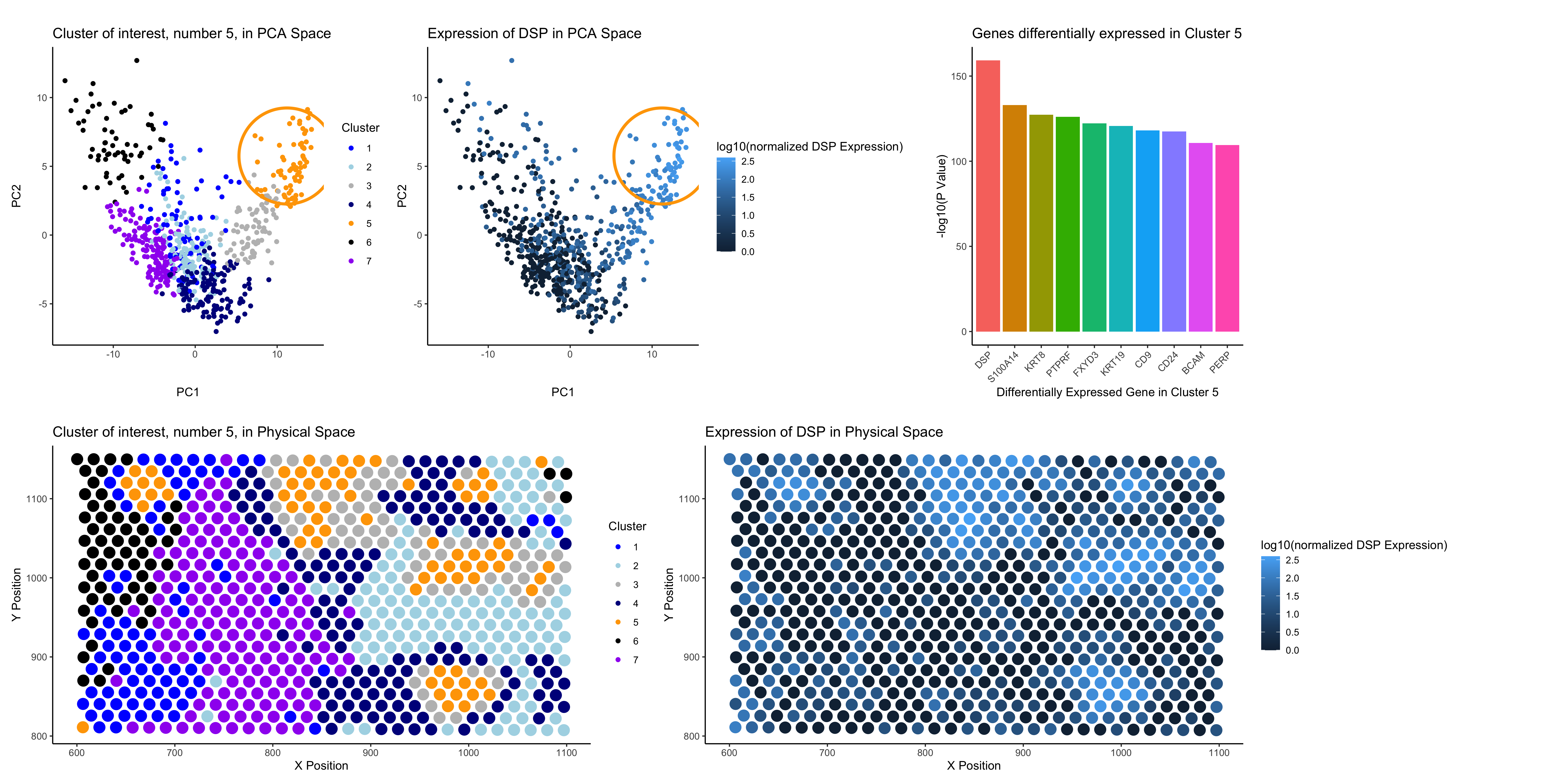
In the top left of my figure, I am depicting both my clusters made by kmeans clustering with k=7 in PCA space (with my cluster of interest circled, cluster 5) and the expression of the most differentially expressed gene in cluster 5 (DSP) in PCA space. Then, on the right of the top row of my figure, I am showing the statistical significance (shown as -log10(p value)) for the top 10 differentially expressed genes in my cluster. Finally, on the bottom row, I am displaying my k-means clusters in physical space and the expression of DSP in physical space as well.
I chose k=7 after graphing the total withiness vs. k values and identified 7 to be the elbow of the graph. I believe that the gene expression of DSP as well as the other top differentially expressed genes in cluster 5 support this choice of k = 7 because the increased expression of these genes is largely confined to the area of cluster 5 in both PCA and physical space.
I believe that cluster 5 are breast granular cells. All of the top 10 differentially expressed genes from cluster 5 that I looked into are found to be expressed at high levels in “breast granular cell” clusters from Protein Atlas, and these clusters on protein Atlas have high expression levels of breast granular cell markers (https://www.proteinatlas.org/ENSG00000096696-DSP/single+cell/breast). Additionally, one of the breast granular cell markers from Protein Atlas, FOXA1, is also significally differentially expressed in my cluster (https://www.proteinatlas.org/ENSG00000096696-DSP/single+cell/breast).
1
2
3
4
5
6
7
8
9
10
11
12
13
14
15
16
17
18
19
20
21
22
23
24
25
26
27
28
29
30
31
32
33
34
35
36
37
38
39
40
41
42
43
44
45
46
47
48
49
50
51
52
53
54
55
56
57
58
59
60
61
62
63
64
65
66
67
68
69
70
71
72
73
74
75
76
77
78
79
80
81
82
83
84
85
86
87
88
89
90
91
92
93
94
95
96
97
98
99
100
101
102
103
104
105
106
107
108
109
110
111
install.packages('patchwork')

file <- '/Users/alexgorham/Desktop/genomic-data-visualization-2025/data/eevee.csv.gz'
data <- read.csv(file)

pos <- data[,3:4]
rownames(pos) <-data$barcode
gexp <- data[,5:ncol(data)]
rownames(gexp) <- data$barcode

topgenes <- names(sort(colSums(gexp),decreasing = TRUE)[1:1000])
gexpsub <- gexp[,topgenes]

norm <- (gexpsub/rowSums(gexpsub))*100000 # per one hundred thousand genes
logexp <- log10(norm+1) #log on the normalized data

ks = c(1, 2, 3, 4, 5, 7, 9, 11, 13, 15, 17, 19, 21, 23, 25, 27, 29, 31, 33, 35)
totw <- sapply(ks, function(k) {
  print(k)
  com <- kmeans(logexp, centers = k) # using the log transformed data
  return(com$tot.withinss)
})
totw
plot(ks, totw)
# determined 7 clusters seems to be the elbow

pcs <- prcomp(logexp)
com <- kmeans(pcs$x[,1:15], centers = 7)
clusters <- com$cluster
names(clusters) <- rownames(gexp)
head(clusters)

interest <- 5
cellsOfInterest <- names(clusters)[clusters == interest]
otherCells <- names(clusters)[clusters != interest]

results <- sapply(1:ncol(logexp), function(i){
  genetest <- logexp[,i]
  names(genetest) <- rownames(logexp)
  out <- t.test(genetest[cellsOfInterest], genetest[otherCells], alternative = 'greater')
  out$p.value
})
names(results) <- colnames(logexp)

library(ggplot2)
df <- data.frame(pcs$x[,1:2], clusters)
panel1 <- ggplot(df, aes(x=PC1, y = PC2, col = factor(clusters))) + geom_point() +
  scale_color_manual(values = c('1' = 'blue',
                                '2' = 'lightblue',
                                '3' = 'grey',
                                '4' = 'darkblue',
                                '5' = 'orange',
                                '6' = 'black',
                                '7' = 'purple')) +
  geom_point(data = df[1, ], aes(x = 11.2, y = 5.75), shape = 1, size = 40, color = "orange", stroke = 2) +
  labs(title = "Cluster of interest, number 5, in PCA Space",
       colour = 'Cluster') +
  theme_classic()

df2 <- data.frame(x = pos$aligned_x, y = pos$aligned_y, clusters)
panel4 <- ggplot(df2, aes(x=x, y = y, col = factor(clusters), size = 0.1)) + geom_point() +
  scale_color_manual(values = c('1' = 'blue',
                                '2' = 'lightblue',
                                '3' = 'grey',
                                '4' = 'darkblue',
                                '5' = 'orange',
                                '6' = 'black',
                                '7' = 'purple')) +
  theme_classic() +
  labs(title = "Cluster of interest, number 5, in Physical Space",
       colour = 'Cluster',
       x = "X Position",
       y = "Y Position") +
  guides(size = "none")

df3 <- data.frame(gene = names(sort(results, decreasing = FALSE)[1:10]), pval = sort(results, decreasing = FALSE)[1:10])
order <- names(sort(results, decreasing = FALSE)[1:10])
df3$gene <- factor(df3$gene, levels = order)

panel3 <- ggplot(df3, aes(x = gene, y = -log10(pval), fill = gene)) +
  geom_col() +
  labs(title = "Genes differentially expressed in Cluster 5",
       x = 'Differentially Expressed Gene in Cluster 5',
       y = '-log10(P Value)') +
  theme_classic() +
  theme(axis.text.x = element_text(angle = 45, hjust = 1)) +
  guides(fill = "none") + theme(plot.margin = margin(20, 100, 20, 20))
panel3

df4 <- data.frame(pcs$x[,1:2], clusters, gene = logexp[,'DSP'])
panel2 <- ggplot(df4, aes(x=PC1, y = PC2, col = gene)) + geom_point() +
  geom_point(data = df[1, ], aes(x = 11.2, y = 5.75), shape = 1, size = 40, color = "orange", stroke = 2) +
  labs(title = "Expression of DSP in PCA Space",
       colour = 'log10(normalized DSP Expression)') +
  theme_classic()

df5 <- data.frame(x = pos$aligned_x, y = pos$aligned_y, clusters, gene = logexp[,'DSP'])
panel5 <- ggplot(df5, aes(x=x, y = y, col = gene, size = 0.1)) + geom_point() +
  theme_classic() +
  labs(title = "Expression of DSP in Physical Space",
       colour = 'log10(normalized DSP Expression)',
       x = "X Position",
       y = "Y Position") +
  guides(size = "none")

library(patchwork)

panels <- (panel1 + panel2 + panel3) / (panel4 + panel5) +
  plot_layout(widths = c(2, 2, 1), heights = c(1, 1))
panels
ggsave("HW3_agorham3.png", panels, width = 20, height = 10, dpi = 300)