
1. Written Answer
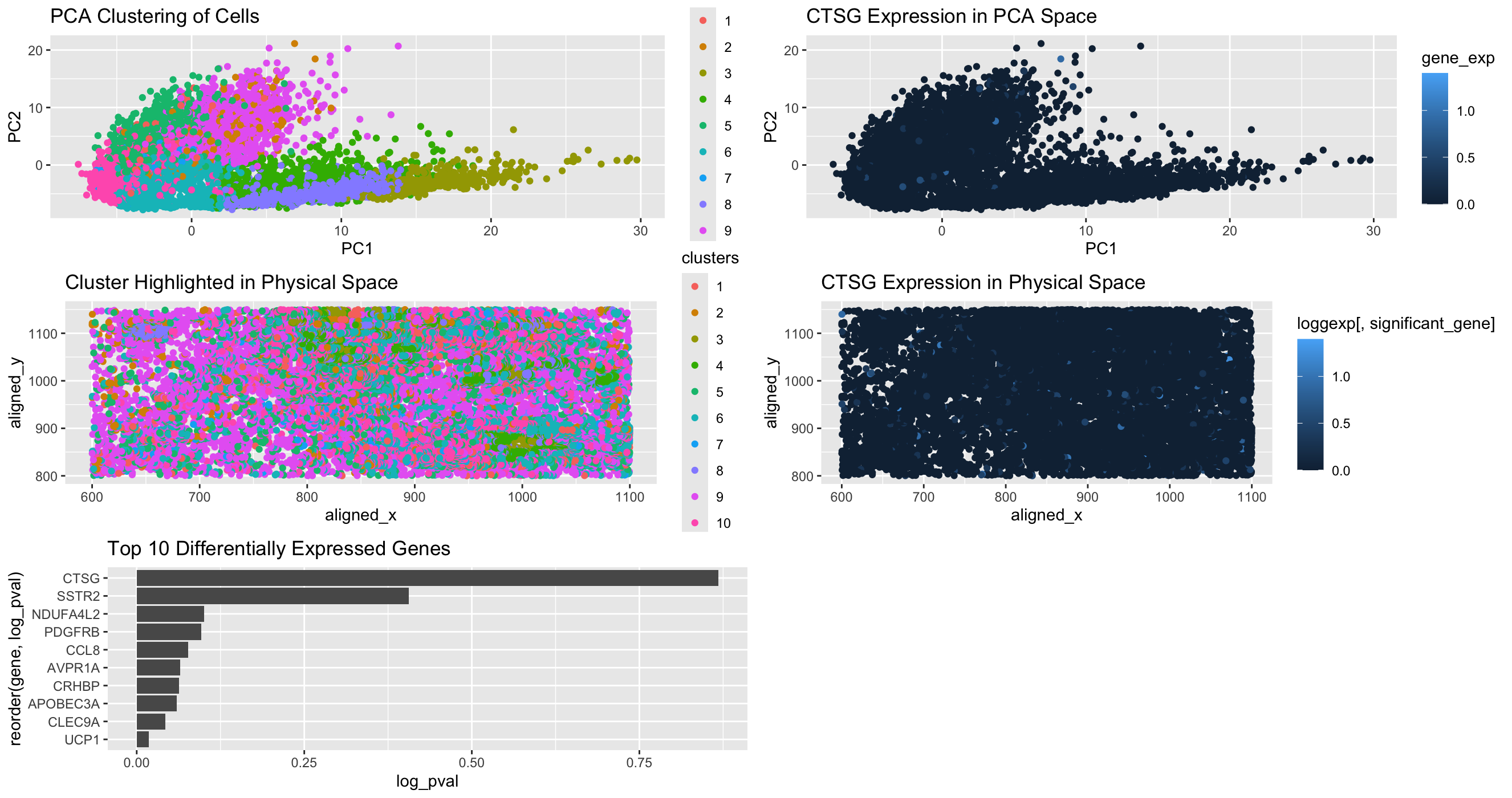
In my data visualization, I made a multi-panel visualization and analysis of cluster 6 which I identified as a transcriptionally distinct population using k-means clustering and PCA. The first panel shows the distribution of the clusters using reduced dimensional space, and you can see cluster 6 as a separate grouping. The second panel uses spatial analysis to highlight the physical location of cluster 6 in the tissue sample. The third panel I made presents the top 10 differentially expressed genes in this cluster using a Wilcoxon test. From this panel, I found that Vimentin (VIM) is upregulated, which was confirmed in panels 4 and 5. In panel 4, the graph shows VIM expression in PCA space and panel 5 shows VIM’s spatial distribution in the tissue. Based on these visualizations and some literature review, I could infer a strong association between cluster 6 and mesenchymal properties.
The expression of VIM strongly suggests that this cluster represents mesenchymal or stromal cells within the breast tissue, specifically cancer associated fibroblasts. Vimentin is a known marker of a process crucial for cancer metastasis known as epithelial to mesenchymal transition. Vimentin is also predominantly expressed in fibroblasts and mesenchymal derived tumors (https://www.proteinatlas.org/ENSG00000026025-VIM). Also, studies have shown that tumor progression is heavily driven by CAFs, promoting metastasis (https://www.nature.com/articles/s41586-018-0641-7). There is a high expression of VIM in cluster 6, and this along with the spatial analysis and physical location provides strong evidence that this cluster is cancer associated stromal cells.
2. Code (paste your code in between the ``` symbols)
1
2
3
4
5
6
7
8
9
10
11
12
13
14
15
16
17
18
19
20
21
22
23
24
25
26
27
28
29
30
31
32
33
34
35
36
37
38
39
40
41
42
43
44
45
46
47
48
49
50
51
52
53
54
55
library(ggplot2)
library(dplyr)
library(tidyr)
library(stats)
library(Rtsne)
library(gridExtra)

file <- '~/Desktop/genomic-data-visualization-2025/data/pikachu.csv.gz'
data <- read.csv(file)

pos <- data[, 5:6]
rownames(pos) <- data$cell_id

gexp <- data[, 7:ncol(data)]
rownames(gexp) <- data$cell_id

loggexp <- log10(gexp + 1)

scaled_gexp <- scale(loggexp)

pca <- prcomp(scaled_gexp)
df_pca <- data.frame(pca$x)
df_pca$cell_id <- rownames(gexp)

set.seed(42)
kmeans_res <- kmeans(scaled_gexp, centers = 10)
clusters <- as.factor(kmeans_res$cluster)
names(clusters) <- rownames(gexp)

df_pca$cluster <- clusters

interest <- 6
cellsOfInterest <- names(clusters)[clusters == interest]
otherCells <- names(clusters)[clusters != interest]

p_values <- sapply(colnames(gexp), function(gene) {
  wilcox.test(gexp[cellsOfInterest, gene], gexp[otherCells, gene], alternative = "greater")$p.value
})

p_values_df <- data.frame(gene = names(p_values), p_value = p_values) %>%
  arrange(p_value) %>%
  mutate(log_pval = -log10(p_value))

significant_gene <- p_values_df$gene[1]

df_pca$gene_exp <- loggexp[, significant_gene]

p1 <- ggplot(df_pca, aes(x = PC1, y = PC2, col = cluster)) + geom_point() + ggtitle("PCA Clustering of Cells")
p2 <- ggplot(df_pca, aes(x = PC1, y = PC2, col = gene_exp)) + geom_point() + ggtitle(paste(significant_gene, "Expression in PCA Space"))
p3 <- ggplot(pos, aes(x = aligned_x, y = aligned_y, col = clusters)) + geom_point() + ggtitle("Cluster Highlighted in Physical Space")
p4 <- ggplot(pos, aes(x = aligned_x, y = aligned_y, col = loggexp[, significant_gene])) + geom_point() + ggtitle(paste(significant_gene, "Expression in Physical Space"))
p5 <- ggplot(p_values_df[1:10, ], aes(x = log_pval, y = reorder(gene, log_pval))) + geom_col() + ggtitle("Top 10 Differentially Expressed Genes")

grid.arrange(p1, p2, p3, p4, p5, ncol = 2)