“Epithelial cell discovery in eevee dataset”

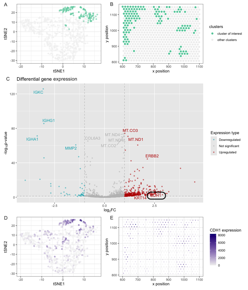
###1. Description Figures A and B share a common legend and analyze the dataset at the cluster level, where green highlights the cluster of interest and gray represents all other clusters. Figure A presents a tSNE plot applied to library size normalized gene expression data, showing that the cluster of interest is distinctly separated from the rest of the cells, however, the cluster itself is dispersed. Figure B visualizes the spatial distribution of the cluster of interest. The tube structure is less obvious compared to pikachu dataset but the cells within this cluster do locate close to each other. Figure C is a volcano plot where red represent up-regulated genes, blue represent down-regulated genes, and try represent non-significant genes. We see that CDH1, a marker gene for epithelial cell, is significantly up-regulated for the cluster of interest indicating that this cluster represent epithelial cells. Both KRT14 and ERBB2 are up-regulated as well, consistent with the previous results from pikachu dataset. Figures D and E analyze CDH1 expression and share a common legend. Figure D displays CDH1 expression on a tSNE plot, where darker blue indicates higher expression, and when compared to Figure A, it is evident that most cells with high CDH1 expression comes from the cluster of interest, however, CDH1 is also expressed in other clusters. Figure E maps CDH1 expression in the physical space, showing a pattern consistent with Figure B. From figure A and C, we see that CDH1 expression is not only expressed in the cluster of interest, and this is likely caused by the limitation of the sequencing method. When using spot approach, although more genes can be analyzed, each spot can contain a mixture of cells, adding noise to the analysis. This effect is also obvious in figure B where the the like structure is lost.
2. Changes
For eve dataset analysis, I used k=8 for k-mean clustering instead of k=6. This is because when plotting k vs. total_withinness, the elbow is at 8 now. I think this is necessary because more genes are being profiled and multiple cell type can exist within one spot. Increases amount of genes and noisiness cause the k to increase to better cluster the data. I also used volcano plot to show the differential expressed gene instead of box plot since it contains more informations.
2. Code
1
2
3
4
5
6
7
8
9
10
11
12
13
14
15
16
17
18
19
20
21
22
23
24
25
26
27
28
29
30
31
32
33
34
35
36
37
38
39
40
41
42
43
44
45
46
47
48
49
50
51
52
53
54
55
56
57
58
59
60
61
62
63
64
65
66
67
68
69
70
71
72
73
74
75
76
77
78
79
80
81
82
83
84
85
86
87
88
89
90
91
92
93
94
95
96
97
98
99
100
101
102
103
104
library(tidyverse)
library(ggplot2)
library(patchwork)
library(DESeq2)
library(ggrepel)
library(Rtsne)

eevee <- read.csv("~/Documents/genom_visual/hw4/eevee.csv")

exp=round(eevee[,-c(1:4)]/rowSums(eevee[,-c(1:4)])*1e7) %>%
  mutate(aligned_x=eevee$aligned_x,
         aligned_y=eevee$aligned_y,
         barcode=eevee$barcode)

selected=names(head(sort(colSums(exp[,1:18085]), decreasing = T), n=5000))

nexp=exp[,c(selected,"aligned_x","aligned_y","barcode")]
row.names(nexp)=nexp$barcode

set.seed(1)
km=kmeans(nexp[,1:5000], centers=8)
clusters <- km$cluster
clusters <- as.factor(clusters)
names(clusters) <- rownames(nexp)
emb <- Rtsne(nexp[,1:5000], )
df <- data.frame(emb$Y)

# plot1
p1=ggplot(df, aes(x=X1, y=X2, colour=ifelse(clusters==1, "in","ot"))) +
  geom_point(alpha=0.5, show.legend = F)+
  xlab("tSNE1")+
  ylab("tSNE2")+
  scale_color_manual(values = c("in" = "aquamarine3", "ot" = "gray94"))+
  theme_bw()


# plot2
p2=cbind(eevee, clusters)%>%
  mutate(clusters=ifelse(clusters==1, "cluster of interest","other clusters"))%>%
  ggplot()+
  geom_point(aes(x = aligned_x, y = aligned_y, colour=clusters), size=2)+
  scale_color_manual(values = c("cluster of interest" = "aquamarine3", "other clusters" = "gray94"))+
  theme_bw()+
  theme(
    panel.grid.major = element_blank(),  # Remove major grid lines
    panel.grid.minor = element_blank()   # Remove minor grid lines
  )+
  xlab("x position")+
  ylab("y position")


c1=nexp[names(clusters)[clusters == 1],"CDH1"]
cr=nexp[names(clusters)[clusters != 1],"CDH1"]

wilcox.test(c1, cr, alternative = 'greater')

group = cbind(nexp, clusters)%>%
  mutate(clusters=ifelse(clusters==1, "B","A"))%>%
  select(barcode, clusters)
vol=t(nexp[,1:5000]) %>%
  as.data.frame()
data=DESeqDataSetFromMatrix(countData = vol, colData = group, design=~clusters)

dds <- results(DESeq(data), tidy=TRUE)

res <- dds %>%
  mutate(padj=ifelse(is.na(padj), pvalue, padj),
         ll=log10(padj),
         degene=ifelse(colnames(nexp[,1:5000]) %in% c("CDH1", "KRT14", "ERBB2", head(dds[order(dds$padj), "row"], 10)),
                       colnames(nexp[,1:5000]), NA),
         type=ifelse(padj<0.5 & log2FoldChange>1, "Up regulated",
                     ifelse(padj<0.5 & log2FoldChange < -1, "Down regulated","Non-significant")))


p3=ggplot(data = res, aes(x = log2FoldChange, y = -log10(padj), colour=type, label=degene))+
  geom_vline(xintercept = c(-1, 1), col = "gray", linetype = 'dashed') +
  geom_hline(yintercept = -log10(0.05), col = "gray", linetype = 'dashed') +
  geom_point(size = 1, alpha=0.5)+
  scale_color_manual(values = c("#00AFBB", "grey", "#bb0c00"),
                     labels = c("Downregulated", "Not significant", "Upregulated"))+
  labs(color = 'Expression type',
       x = expression("log"[2]*"FC"), y = expression("-log"[10]*"p-value"))+
  ggtitle('Differential gene')+
  geom_text_repel(max.overlaps = Inf, show.legend = F)

p4=ggplot(df, aes(x=X1, y=X2, colour=nexp[,"CDH1"]+1)) +
  geom_point(alpha=0.5, show.legend = F)+
  xlab("tSNE1")+
  ylab("tSNE2")+
  scale_color_gradient(low="gray94", high="navy")+
  theme_bw()


p5 = nexp%>%
  ggplot()+
  geom_point(aes(x = aligned_x, y = aligned_y, colour=CDH1), size=0.4, alpha=0.8)+
  scale_color_gradient(low="gray94", high="navy")+
  theme_bw()+
  labs(colour = "CDH1 expression")+
  xlab("x position")+
  ylab("y position")


(p1+p2)/p3/(p4+p5) + plot_layout(heights = c(1,2,1))