Description

Notes: I want to change the cluster identified in HW3. Originally, it is most likely a fibroblast-like stromal cell because the top 20 highly expressed genes include SFRP4, WIF1, CHI3L1, PTX3, and MMRN1, which are associated with ECM remodeling, Wnt signaling inhibition, and inflammatory responses. These features are commonly found in tumor-associated fibroblasts (CAFs) and mesenchymal stromal cells. However, most of the top 20 highly expressed genes in this cluster are not even present in the Pikachu dataset. Therefore, I have decided to focus on identifying epithelial cells in both datasets (the new codes for the Eevee dataset are attached below).

Core epithelial markers include EPCAM, CDH1, DSP, TACSTD2, and keratin (KRT) families (Karantza, 2011). For example, KRT8, KRT18, and KRT19 are simple epithelial cytokeratins, typically found in glandular and luminal epithelial cells, whereas KRT5 and KRT14 are basal epithelial markers, commonly associated with stratified epithelium.

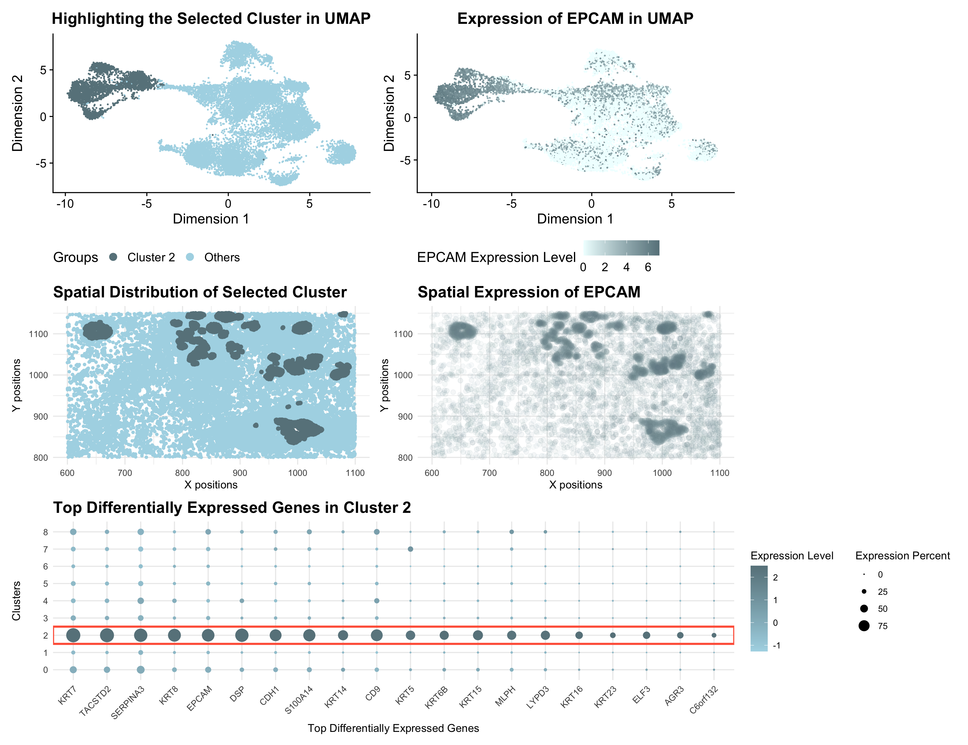
The Pikachu dataset-based visualizations provide a comprehensive representation of Cluster 2 and its association with EPCAM, combining UMAP, spatial, and gene expression analysis. The top-left UMAP plot highlights Cluster 2 (dark gray) as a distinct group within the low-dimensional space, setting it apart from other clusters (light blue). EPCAM is a well-known epithelial marker, and the top-right UMAP plot further illustrates that its expression is enriched in specific regions, suggesting a strong association with Cluster 2.

In the spatial analysis, the bottom-left panel shows the physical distribution of Cluster 2 cells within the 2D tissue space, revealing a clear localization pattern. Similarly, the bottom-right spatial expression plot confirms that EPCAM is expressed in the same region, reinforcing its biological relevance to this cluster. Finally, the bottom dot plot displays the top differentially expressed genes in Cluster 2, where the top 20 highly expressed genes are listed (most of them associated with epithelial cells, as discussed above). The dot size represents the percentage of cells expressing each gene, while the color gradient indicates expression intensity.

Together, these visualizations strongly suggest that Cluster 2 represents epithelial cells. I also examined the expression of these top 20 highly expressed genes in the Eevee dataset, where they show distinctly high expression in Cluster 2 compared to other clusters. This finding suggests that they likely represent the same cell type in both datasets.

I previously performed k-means clustering with k = 4, but I have now repeated the analysis using k = 9 because I determined the optimal K for this dataset based on total within-cluster variance (total withinness) to be 9. I believe that the optimal number of transcriptionally distinct cell clusters is lower in the spot-based Eevee dataset compared to the single-cell resolution Pikachu dataset, possibly because the Pikachu dataset captures the finer granularity of gene expression differences between individual cells, allowing for more distinct transcriptional clusters. The increased within-spot averaging in the Eevee dataset likely results in fewer clearly separable clusters, as transcriptional profiles are blended across multiple cells. Additionally, spatial transcriptomics datasets often exhibit higher technical noise and spatially driven expression patterns, which might further contribute to a lower optimal K compared to single-cell RNA-seq data.

Reference: Karantza V. Keratins in health and cancer: more than mere epithelial cell markers. Oncogene. 2011 Jan 13;30(2):127-38. doi: 10.1038/onc.2010.456. Epub 2010 Oct 4. PMID: 20890307; PMCID: PMC3155291.

library(Seurat)
library(ggplot2)
library(patchwork)
library(dplyr)

##############
data = read.csv('/Users/yiyang/Downloads/pikachu.csv.gz')
metadata <- data[, c("X","cell_id","cell_area","nucleus_area", "aligned_x", "aligned_y")]
rownames(metadata) <- metadata$barcode
data <- data[, !colnames(data) %in% c("X","cell_id","cell_area","nucleus_area", "aligned_x", "aligned_y")]
##############
seurat_obj <- CreateSeuratObject(counts = t(data), meta.data = metadata)
seurat_obj <- NormalizeData(seurat_obj)
seurat_obj <- FindVariableFeatures(seurat_obj, selection.method = "vst", nfeatures = 2000)
seurat_obj <- ScaleData(seurat_obj)
seurat_obj <- RunPCA(seurat_obj, features = VariableFeatures(object = seurat_obj))
seurat_obj <- RunUMAP(seurat_obj, dims = 1:30)
seurat_obj <- FindNeighbors(seurat_obj, dims = 1:30)
seurat_obj <- FindClusters(seurat_obj, resolution = 0.1)
DimPlot(seurat_obj, reduction = "umap", label = TRUE, pt.size = 0.5) + NoLegend()

# Highlighting one cluster of interest 

seurat_obj$cluster_highlight <- ifelse(Idents(seurat_obj) == "2", "Cluster 2", "Others")
selected_cluster_colors <- c("Cluster 2"="#68838B","Others"="#ADD8E6")
title_theme <- theme(plot.title = element_text(size = 16, face = "bold"))
p1 <- DimPlot(seurat_obj, reduction = "umap", group.by = "cluster_highlight") + 
  ggtitle("Highlighting the Selected Cluster in UMAP") + labs(x = "Dimension 1", y = "Dimension 2") + 
  scale_color_manual(values = selected_cluster_colors,name = "Groups") + title_theme + 
  theme(legend.position = "bottom")
p2 <- ggplot() +
  geom_point(data = metadata %>% filter(Idents(seurat_obj) != "2"), 
             aes(x = aligned_x, y = aligned_y), 
             color = "#ADD8E6", size = 1) + 
  geom_point(data = metadata %>% filter(Idents(seurat_obj) == "2"), 
             aes(x = aligned_x, y = aligned_y), 
             color = "#68838B", size = 1.5) +  
  theme_minimal() +
  scale_color_manual(values = c("#ADD8E6", "#68838B"), 
                     labels = c("Other Clusters", "Cluster 2"), 
                     name = "Cluster Identity") +
  ggtitle("Spatial Distribution of Selected Cluster") + 
  labs(x = "X positions", y = "Y positions") + title_theme 

# Find markers for the selected cluster 
cluster_of_interest <- "2"
markers_cluster <- FindMarkers(seurat_obj, ident.1 = cluster_of_interest, min.pct = 0.25, logfc.threshold = 0.25)
top_gene <- rownames(markers_cluster)[1]  
top_gene = "EPCAM"
p3 = FeaturePlot(seurat_obj, features = top_gene) + 
  ggtitle(paste("Expression of", top_gene, "in UMAP")) + labs(x = "Dimension 1", y = "Dimension 2") +
  scale_color_gradientn(colors = c("#F0FFFF","#68838B"), name = "EPCAM Expression Level") + title_theme + 
  theme(legend.position = "bottom")
# Create a volcano plot
top_genes <- rownames(markers_cluster[order(markers_cluster$avg_log2FC, decreasing = TRUE),])[1:20]  # Top 10 genes
avg_exp <- AverageExpression(seurat_obj, features = top_genes)$RNA
avg_exp_df <- as.data.frame(avg_exp)
avg_exp_df$gene <- rownames(avg_exp_df)
top_genes_ordered <- avg_exp_df$gene[order(rowMeans(avg_exp_df[,-ncol(avg_exp_df)]), decreasing = TRUE)]
p4 = DotPlot(seurat_obj, features = top_genes_ordered, cols = c("#ADD8E6", "#68838B")) +
  ggtitle("Top Differentially Expressed Genes in Cluster 2") +
  theme_minimal() + labs(x = "Top Differentially Expressed Genes", y = "Clusters") + 
  theme(axis.text.x = element_text(angle = 45, hjust = 1)) + 
  annotate("rect", 
           xmin = -Inf, xmax = Inf, 
           ymin = 3 - 0.5,
           ymax = 3 + 0.5,
           color = "#FF6347", fill = NA, size = 1) + title_theme +
  guides(color = guide_colorbar(order = 1, title = "Expression Level"), size = guide_legend(order = 2, title = "Expression Percent")) +  
  theme(
    legend.position = "right",
    legend.box = "horizontal" 
  )


metadata$EPCAM <- FetchData(seurat_obj, vars = "EPCAM")$EPCAM
metadata <- metadata[order(metadata$EPCAM), ]
p5 <- ggplot(metadata, aes(x = aligned_x, y = aligned_y, color = EPCAM, alpha = EPCAM)) +
  geom_point(size = 2) +  
  scale_color_gradientn(colors = c("#F0FFFF", "#68838B"), name = "EPCAM Expression") +  
  scale_alpha(range = c(0, 0.2)) +  guides(alpha = "none") +
  theme_minimal() +
  ggtitle("Spatial Expression of EPCAM") +
  labs(x = "X positions", y = "Y positions") + 
  title_theme + theme(legend.position = "none")

s = (p1 | p3) / (p2 | p5) / p4 


####################################
data_eevee = read.csv('/Users/yiyang/Downloads/eevee.csv.gz')
metadata_eevee <- data_eevee[, c("barcode", "aligned_x", "aligned_y")]
rownames(metadata_eevee) <- metadata_eevee$barcode
data_eevee <- data_eevee[, !colnames(data_eevee) %in% c("barcode", "aligned_x", "aligned_y")]
seurat_obj_eevee <- CreateSeuratObject(counts = t(data_eevee), meta.data = metadata_eevee)
seurat_obj_eevee <- NormalizeData(seurat_obj_eevee)
seurat_obj_eevee <- FindVariableFeatures(seurat_obj_eevee, selection.method = "vst", nfeatures = 2000)
seurat_obj_eevee <- ScaleData(seurat_obj_eevee)
seurat_obj_eevee <- RunPCA(seurat_obj_eevee, features = VariableFeatures(object = seurat_obj_eevee))
seurat_obj_eevee <- RunUMAP(seurat_obj_eevee, dims = 1:30)
seurat_obj_eevee <- FindNeighbors(seurat_obj_eevee, dims = 1:30)
seurat_obj_eevee <- FindClusters(seurat_obj_eevee, resolution = 0.4)
# Highlighting one cluster of interest (cluster 0)
seurat_obj_eevee$cluster_highlight <- ifelse(Idents(seurat_obj_eevee) == "2", "Cluster 2", "Others")
selected_cluster_colors_eevee <- c("Cluster 2"="#68838B","Others"="#ADD8E6")
title_theme_eevee <- theme(plot.title = element_text(size = 16, face = "bold"))
p1_eevee <- DimPlot(seurat_obj_eevee, reduction = "umap", group.by = "cluster_highlight") + 
  ggtitle("Highlighting the Selected Cluster in UMAP") + labs(x = "Dimension 1", y = "Dimension 2") + 
  scale_color_manual(values = selected_cluster_colors_eevee,name = "Groups") + title_theme_eevee
p2_eevee <- ggplot(metadata_eevee, 
             aes(x = aligned_x, 
                 y = aligned_y,
                 color = ifelse(as.factor(Idents(seurat_obj_eevee)) == "2", 
                                "Cluster 2", "Other Clusters"))) +
  geom_point() +
  scale_color_manual(values = c("Cluster 2" = "#68838B", "Other Clusters" = "#ADD8E6"),name = "Groups") +
  theme_minimal() + 
  ggtitle("Spatial Distribution of Selected Cluster") + labs(x = "X positions", y = "Y positions") + title_theme_eevee
# Find markers for the selected cluster (cluster 0)
cluster_of_interest_eevee <- "2"
markers_cluster_eevee <- FindMarkers(seurat_obj_eevee, ident.1 = cluster_of_interest_eevee, min.pct = 0.25, logfc.threshold = 0.25)
top_gene_eevee <- rownames(markers_cluster_eevee)[1]  
p3_eevee = FeaturePlot(seurat_obj_eevee, features = top_gene_eevee) + 
  ggtitle(paste("Expression of", top_gene_eevee, "in UMAP")) + labs(x = "Dimension 1", y = "Dimension 2") +
  scale_color_gradientn(colors = c("#F0FFFF","#68838B"), name = "SFRP4 Expression Level") + title_theme_eevee
# Create a volcano plot
top_genes_eevee <- rownames(markers_cluster_eevee[order(markers_cluster_eevee$avg_log2FC, decreasing = TRUE),])[1:10]  # Top 10 genes
avg_exp_eevee <- AverageExpression(seurat_obj_eevee, features = top_genes_eevee)$RNA
avg_exp_df_eevee <- as.data.frame(avg_exp_eevee)
avg_exp_df_eevee$gene <- rownames(avg_exp_df_eevee)
top_genes_ordered_eevee <- avg_exp_df_eevee$gene[order(rowMeans(avg_exp_df_eevee[,-ncol(avg_exp_df_eevee)]), decreasing = TRUE)]
p4_eevee = DotPlot(seurat_obj_eevee, features = top_genes_ordered_eevee , cols = c("#ADD8E6", "#68838B")) +
  ggtitle("Top Differentially Expressed Genes in Cluster 2 (eevee dataset)") +
  theme_minimal() + labs(x = "Top Differentially Expressed Genes", y = "Clusters") + 
  theme(axis.text.x = element_text(angle = 45, hjust = 1)) + 
  # annotate("rect", 
  #          ymin = 3 - 0.5, 
  #          ymax = 3 + 0.5, 
  #          xmin = -Inf, xmax = Inf, 
  #          color = "#FF6347", fill = NA, size = 1) + 
  title_theme_eevee +
  guides(color = guide_colorbar(order = 1, title = "Expression Level"), size = guide_legend(order = 2, title = "Expression Percent")) +  
  theme(
    legend.position = "right",
    legend.box = "horizontal" 
  )
metadata_eevee$KRT7 <- FetchData(seurat_obj_eevee, vars = "KRT7")$KRT7
metadata_eevee <- metadata_eevee[order(metadata_eevee$KRT7), ]
p5_eevee <- ggplot(metadata_eevee, aes(x = aligned_x, y = aligned_y, color = KRT7)) +
  geom_point(size = 2) +  
  scale_color_gradientn(colors = c("#F0FFFF", "#68838B"), name = "KRT7 Expression") +  
  theme_minimal() +
  ggtitle("Spatial Expression of KRT7") +
  labs(x = "X positions", y = "Y positions") + 
  title_theme_eevee
s2 = (p1_eevee | p3_eevee) / (p2_eevee | p5_eevee) / p4_eevee