Identifying the same cluster of cells within the Eevee dataset

1. Write a description explaining why you believe your data visualization is effective using vocabulary terms from Lesson 1.
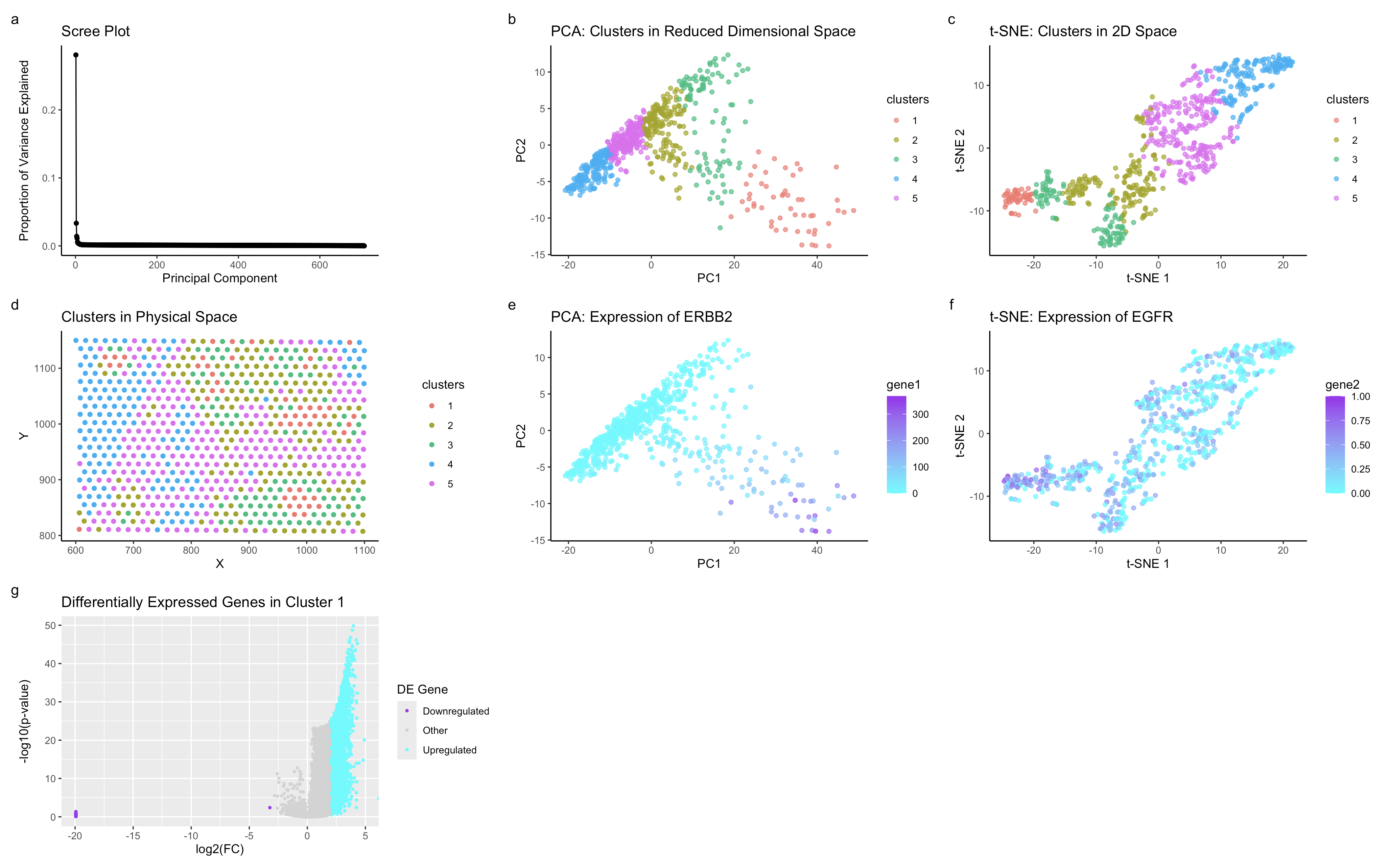
Applying the same analytical approach from HW3, I identified a corresponding cell type in the HW4 dataset by leveraging dimensionality reduction, clustering, and spatial gene expression analysis. In HW3, I characterized a distinct olive-colored cluster, which exhibited a unique transcriptional profile and spatial organization, strongly suggesting that it represented luminal epithelial cells engaged in growth factor signaling. This conclusion was based on the co-expression of ERBB2 and EGFR, two hallmark epithelial markers, along with CDH1 and FOXA1, further supporting its identity as an epithelial population involved in tissue maintenance or regeneration.
To confirm the presence of this same cell type in HW4, I re-applied k-means clustering, PCA, and t-SNE to the new dataset. The PCA (b) and t-SNE (c) plots in HW4 revealed a cluster with a similar transcriptional identity and structure to the olive cluster from HW3, suggesting a preserved biological population across datasets. Additionally, the physical space visualization (d) in HW4 indicates that this cluster maintains an organized spatial distribution, reinforcing the idea that it is a biologically meaningful group rather than a computational artifact.
Gene expression analysis further validates this finding. The PCA and t-SNE expression plots (e, f) in HW4 show that ERBB2 and EGFR are highly expressed in the same distinct cluster, mirroring their localization in HW3. Moreover, spatial expression plots (g, h) confirm that this population is non-randomly distributed in tissue space, further supporting the hypothesis that it represents an epithelial cell type engaged in active signaling.
Finally, the differential gene expression analysis in HW4 (g) provides strong statistical support for this cluster’s unique transcriptional identity. The volcano plot highlights significantly upregulated genes in the cluster, which may align with the transcriptional signature observed in HW3.
2. Code (paste your code in between the ``` symbols)
1
2
3
4
5
6
7
8
9
10
11
12
13
14
15
16
17
18
19
20
21
22
23
24
25
26
27
28
29
30
31
32
33
34
35
36
37
38
39
40
41
42
43
44
45
46
47
48
49
50
51
52
53
54
55
56
57
58
59
60
61
62
63
64
65
66
67
68
69
70
71
72
73
74
75
76
77
78
79
80
81
82
83
84
85
86
87
88
89
90
91
92
93
94
95
96
97
98
99
100
101
102
103
104
105
106
107
108
109
110
111
112
113
114
115
116
117
118
119
120
121
122
123
124
125
126
127
128
129
130
131
132
133
134
135
136
137
138
139
140
141
142
143
144
145
146
147
148
149
150
# Load Required Libraries
library(Rtsne)
library(ggplot2)
library(patchwork)
library(cluster)

# Load Data
eevee_file <- "~/code/genomic-data-visualization-2025/data/eevee.csv.gz"
data <- read.csv(eevee_file)

# Extract Position & Gene Expression Data
pos <- data[, 3:4]
colnames(pos) <- c("X1", "X2")  # Ensure correct column names
rownames(pos) <- data$X

gexp <- data[, 5:ncol(data)]  # Extract gene expression
rownames(gexp) <- data$X  # Align gene expression with sample names

# Normalize Gene Expression
norm <- gexp / rowSums(gexp) * 10000
topgenes <- names(sort(colSums(norm), decreasing = TRUE)[1:1000])
normsub <- norm[, topgenes]

# Log Transformation
gexp_log <- log10(gexp + 1)

# K-Means Clustering
set.seed(123)
clusters <- kmeans(gexp_log, centers = 5)$cluster
clusters <- as.factor(clusters)
names(clusters) <- rownames(gexp)

# PCA
pcs <- prcomp(gexp_log)
df_pca <- data.frame(pcs$x, clusters)

# t-SNE using top 10 PCs
set.seed(123)
tsne_emb <- Rtsne(pcs$x[, 1:10], dims = 2, perplexity = 50)$Y
df_tsne <- data.frame(tsne_emb, clusters)
colnames(df_tsne) <- c("X1", "X2", "clusters")

# Scree Plot (Variance Explained)
variance_explained <- pcs$sdev^2
total_variance <- sum(variance_explained)
proportion_variance_explained <- variance_explained / total_variance
pc_data <- data.frame(PC_Number = 1:length(proportion_variance_explained),
                      ProportionVariance = proportion_variance_explained)

p_scree <- ggplot(pc_data, aes(x = PC_Number, y = ProportionVariance)) +
  geom_line() +
  geom_point() +
  labs(title = "Scree Plot", x = "Principal Component", y = "Proportion of Variance Explained") +
  theme_classic()

# PCA - Cluster Visualization
p_pca_clusters <- ggplot(df_pca, aes(x = PC1, y = PC2, col = clusters)) +
  geom_point(alpha = 0.7) +
  labs(title = 'PCA: Clusters in Reduced Dimensional Space', x = "PC1", y = "PC2") +
  theme_classic()

# t-SNE - Cluster Visualization
p_tsne_clusters <- ggplot(df_tsne, aes(x = X1, y = X2, col = clusters)) +
  geom_point(alpha = 0.7) +
  labs(title = 't-SNE: Clusters in 2D Space', x = "t-SNE 1", y = "t-SNE 2") +
  theme_classic()

# Physical Space - Cluster Visualization
p_physical_space <- ggplot(data.frame(pos, clusters)) +
  geom_point(aes(x = X1, y = X2, col = clusters)) +
  labs(title = 'Clusters in Physical Space', x = "X", y = "Y") +
  theme_classic()

# Differential Expression for Specific Genes (Ensure Gene Exists)
gene_interest1 <- 'ERBB2'
if (gene_interest1 %in% colnames(gexp)) {
  df_pca$gene1 <- gexp[, gene_interest1]

  p_gene_pca <- ggplot(df_pca, aes(x = PC1, y = PC2, col = gene1)) +
    geom_point(alpha = 0.7) +
    labs(title = paste('PCA: Expression of', gene_interest1), x = "PC1", y = "PC2") +
    scale_color_gradient(low = "cyan", high = "purple") +
    theme_classic()
} else {
  print(paste("Warning: Gene", gene_interest1, "not found in dataset."))
  p_gene_pca <- NULL
}

# t-SNE Expression Visualization for EGFR (Ensure Gene Exists)
gene_interest2 <- 'EGFR'
if (gene_interest2 %in% colnames(gexp_log)) {
  df_tsne$gene2 <- gexp_log[, gene_interest2]

  p_gene_tsne1 <- ggplot(df_tsne, aes(x = X1, y = X2, col = gene2)) +
    geom_point(alpha = 0.7) +
    labs(title = 't-SNE: Expression of EGFR', x = "t-SNE 1", y = "t-SNE 2") +
    scale_color_gradient(low = "cyan", high = "purple") +
    theme_classic()
} else {
  print(paste("Warning: Gene", gene_interest2, "not found in dataset."))
  p_gene_tsne1 <- NULL
}

# Create Volcano Plot Data
df_volc <- data.frame(pvalues = -log10(filtered_pvalues), log_fc = filtered_logfc)
df_volc$genes <- rownames(df_volc)

# Define thresholds
upper_logfc <- 2
lower_logfc <- -3

df_volc$color <- ifelse(df_volc$log_fc > upper_logfc, "Upregulated",
                        ifelse(df_volc$log_fc < lower_logfc, "Downregulated", "Other"))

# Volcano Plot
p_volcano <- ggplot(df_volc, aes(x = log_fc, y = pvalues, color = color)) +
  geom_point(size = 0.75) +
  ggtitle("Differentially Expressed Genes in Cluster 5") +
  scale_color_manual(values = c("Upregulated" = "cyan",
                                "Downregulated" = "purple",
                                "Other" = "lightgray")) +
  labs(color = "DE Gene") +
  xlab("log2(FC)") +
  ylab("-log10(p-value)")


# Combine Plots
combined_plot <- p_scree + p_pca_clusters + p_tsne_clusters + p_physical_space +
  p_gene_pca + p_gene_tsne1 + p_volcano + plot_annotation(tag_levels = 'a') +
  plot_layout(ncol = 3)

print(combined_plot)

# Identify Top Genes
olive_cluster_cells <- rownames(df_pca[df_pca$clusters == "1", ])
olive_cluster_expression <- colMeans(gexp_log[olive_cluster_cells, ])
other_clusters_expression <- colMeans(gexp_log[-which(rownames(gexp_log) %in% olive_cluster_cells), ])
log2fc <- log2(olive_cluster_expression + 1) - log2(other_clusters_expression + 1)
top_olive_genes <- sort(log2fc, decreasing = TRUE)[1:20]  # Top 20 most overexpressed genes
print("Top Overexpressed Genes in Olive Cluster:")
print(top_olive_genes)

# Identify Most Variable Genes
var_olive <- apply(gexp_log[olive_cluster_cells, ], 2, var)
other_cells <- setdiff(rownames(gexp_log), olive_cluster_cells)
var_other <- apply(gexp_log[other_cells, ], 2, var)
var_ratio <- var_olive / (var_other + 1e-6)  # Avoid division by zero
top_variable_genes <- names(sort(var_ratio, decreasing = TRUE))[1:20]  # Top 20 most variable genes
print("Top Most Variable Genes in Olive Cluster:")
print(top_variable_genes)