Hw4: Finding the same cell cluster in the other dataset

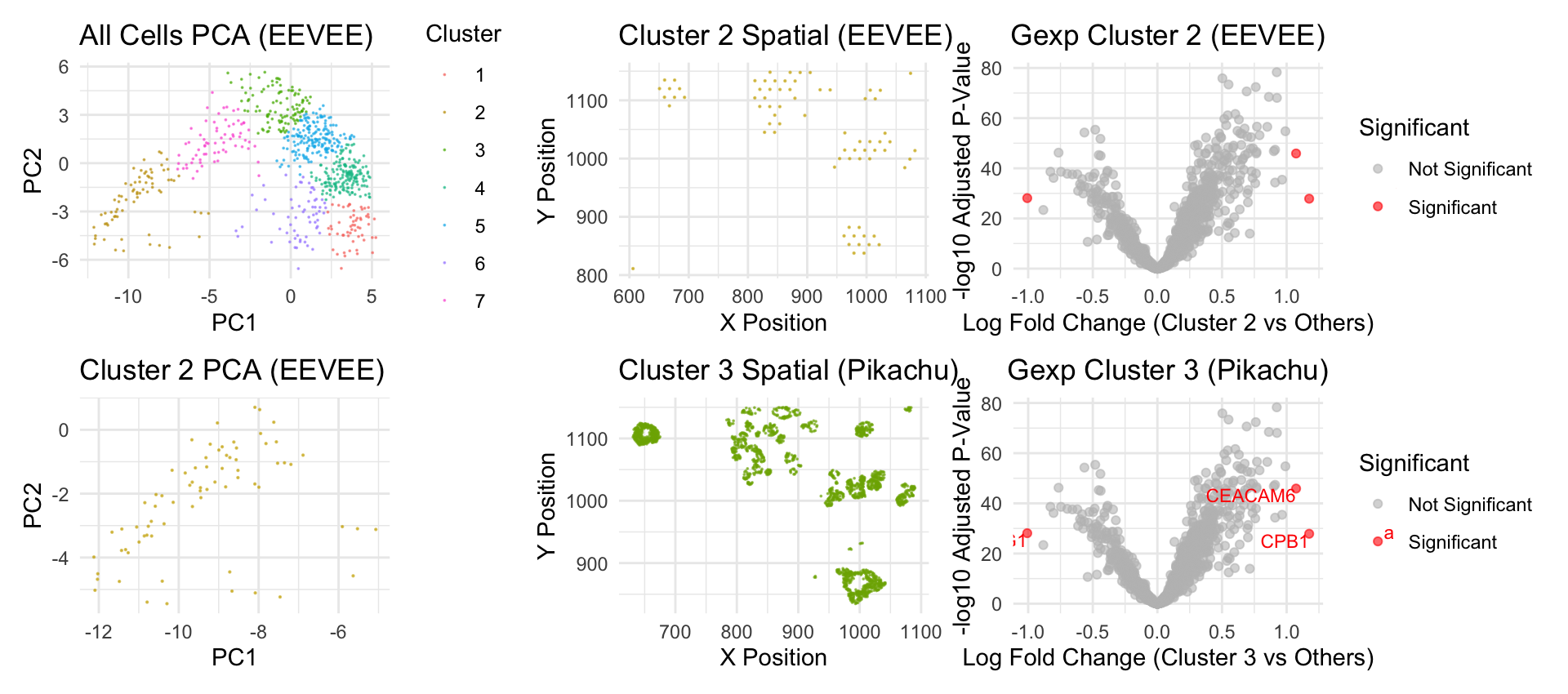
This panel shows that the cell cluster that I found in the EEVEE dataset is the same that I had found in the Pikachu dataset for the previous homework. The first graph in the panel shows all the spots in the EEVEE dataset in the PCA space. I chose cluster 2 to look at more closely because the spatial distribution of this cluster in the EEVEE dataset was very similar to the spatial distribution of cluster 3 in the Pikachu dataset. This similarity can be viewed by graphs 2 and 5 in the panel. Since the EEVEE dataset is from sequencing data, it’s not at the single molecule level so the spots are more generalized than the Pikachu data. Next, I compared the gene expressions of both datasets at their respective clusters using a volcano plot. The plots came out very similar, with the same three genes being significantly differentially expressed between the cells of interest and others. Using these observations, I came to the conclusion that the cells in cluster 2 in the EEVEE dataset are of the same type of the cells in cluster 3 in the Pikachu dataset.
5. Code (paste your code in between the ``` symbols)
1
2
3
4
5
6
7
8
9
10
11
12
13
14
15
16
17
18
19
20
21
22
23
24
25
26
27
28
29
30
31
32
33
34
35
36
37
38
39
40
41
42
43
44
45
46
47
48
49
50
51
52
53
54
55
56
57
58
59
60
61
62
63
64
65
66
67
68
69
70
71
72
73
74
75
76
77
78
79
80
81
82
83
84
85
86
87
88
89
90
91
92
93
94
95
96
97
98
99
100
101
102
103
104
105
106
107
108
109
110
111
112
113
114
115
116
117
118
119
120
121
122
123
124
125
126
127
128
129
130
131
132
133
134
135
136
137
138
139
140
141
142
143
144
145
146
147
148
149
150
151
152
153
154
155
156
157
158
159
160
161
162
163
164
165
166
167
168
169
170
171
172
173
174
175
176
## EEVEE
file <- '/Users/anishkabhartiya/Desktop/genomic-data-visualization-2025/data/eevee.csv.gz'
data <- read.csv(file)
data[1:5, 1:10]

pos <- data[, 3:4]
rownames(pos) <- data$barcode
head(pos)
gexp <- data[, 5:ncol(data)]
rownames(gexp) <- data$barcode
gexp[1:5,1:5]
dim(gexp)

topgenes <- names(sort(colSums(gexp), decreasing=TRUE)[1:2000])
gexpsub <- gexp[,topgenes]
gexpsub[1:5,1:5]
dim(gexpsub)

norm <- gexpsub/rowSums(gexpsub) * 10000
norm[1:5,1:5]
norm <- log10(norm + 1)

pcs <- prcomp(norm)
set.seed(1)


pca_df <- data.frame(
  PC1 = pcs$x[,1],
  PC2 = pcs$x[,2],
  X = data[,3],
  Y = data[,4]
)

clusters <- kmeans(pca_df[,1:2], centers = 7)$cluster


pca_df$Cluster <- as.factor(clusters)
pca_df_filtered <- pca_df[pca_df$Cluster == "2", ]
cellsOfInterest <- rownames(pca_df)[pca_df$Cluster == "2"]
otherCells <- rownames(pca_df)[pca_df$Cluster != "2"]

p_values <- apply(norm, 2, function(gene) {
  t.test(gene[cellsOfInterest], gene[otherCells])$p.value
})

logFC <- colMeans(norm[cellsOfInterest, ]) - colMeans(norm[otherCells, ])
adjusted_p_values <- p.adjust(p_values, method = "fdr")  # Adjust for multiple testing

volcano_df <- data.frame(
  Gene = colnames(norm),
  LogFC = logFC,
  p_value = p_values,
  neg_log10_p = -log10(adjusted_p_values)
)

volcano_df$Significant <- ifelse(volcano_df$p_value < 0.05 & abs(volcano_df$LogFC) > 1, "Significant", "Not Significant")


library(ggplot2)
library(patchwork)

g1 <- ggplot(pca_df, aes(x = PC1, y = PC2, color = Cluster)) +
  geom_point(alpha = 0.6, size=0.01) +
  labs(title = "All Cells PCA (EEVEE)",
       x = "PC1",
       y = "PC2") +
  theme_minimal()

g2 <- ggplot(pca_df_filtered, aes(x = PC1, y = PC2, color = Cluster)) +
  geom_point(alpha = 0.6, size=0.1, color = 'gold3') +
  labs(title = "Cluster 2 PCA (EEVEE)",
       x = "PC1",
       y = "PC2") +
  theme_minimal() +
  theme(legend.position = "none")

g3 <- ggplot(pca_df_filtered, aes(x = X, y = Y, color = Cluster)) +
  geom_point(alpha = 0.6, size=0.1, color = 'gold3') +
  labs(title = "Cluster 2 Spatial (EEVEE)",
       x = "X Position",
       y = "Y Position") +
  theme_minimal() +
  theme(legend.position = "none")

g4 <- ggplot(volcano_df, aes(x = LogFC, y = neg_log10_p, color = Significant)) +
  geom_point(alpha = 0.6) +
  scale_color_manual(values = c("Significant" = "red", "Not Significant" = "gray")) +
  geom_text(data = subset(volcano_df, Significant == "Significant" & neg_log10_p > 2),
            aes(label = Gene), vjust = 1, hjust = 1, size = 0.1) +
  theme_minimal() +
  labs(title = "Gexp Cluster 2 (EEVEE)",
       x = "Log Fold Change (Cluster 2 vs Others)",
       y = "-log10 Adjusted P-Value") +
  theme(plot.title = element_text(hjust = 0.5))

significant_genes <- volcano_df[volcano_df$Significant == "Significant", "Gene"]

top_significant_genes <- head(significant_genes[order(volcano_df$p_value[volcano_df$Significant == "Significant"])], 20)
print(top_significant_genes)

##PIKACHU

file <- '/Users/anishkabhartiya/Desktop/genomic-data-visualization-2025/data/pikachu.csv.gz'
data <- read.csv(file)
data[1:5, 1:10]

area <- data[, 3:4]
pos <- data[, 5:6]
rownames(pos) <- data$barcode
head(pos)
gexp <- data[, 7:ncol(data)]
rownames(gexp) <- data$barcode
gexp[1:5,1:5]
dim(gexp)

norm <- gexp / log10(data$cell_area+1) * 3
norm[1:5, 1:5]

pcs <- prcomp(norm)
set.seed(1)


pca_df <- data.frame(
  PC1 = pcs$x[,1],
  PC2 = pcs$x[,2],
  X = data[,5],
  Y = data[,6]
)

clusters <- kmeans(pca_df[,1:2], centers = 7)$cluster


pca_df$Cluster <- as.factor(clusters)
pca_df_filtered <- pca_df[pca_df$Cluster == "3", ]
cellsOfInterest <- rownames(pca_df)[pca_df$Cluster == "3"]
otherCells <- rownames(pca_df)[pca_df$Cluster != "3"]

library(ggplot2)

p_values <- apply(norm, 2, function(gene) {
  t.test(gene[cellsOfInterest], gene[otherCells])$p.value
})

logFC <- colMeans(norm[cellsOfInterest, ]) - colMeans(norm[otherCells, ])

adjusted_p_values <- p.adjust(p_values, method = "fdr")

volcano_df <- data.frame(
  Gene = colnames(norm),
  LogFC = logFC,
  p_value = p_values,
  neg_log10_p = -log10(adjusted_p_values)
)

volcano_df$Significant <- ifelse(volcano_df$p_value < 0.05 & abs(volcano_df$LogFC) > 1, "Significant", "Not Significant")

g5 <- ggplot(volcano_df, aes(x = LogFC, y = neg_log10_p, color = Significant)) +
  geom_point(alpha = 0.6) +
  scale_color_manual(values = c("Significant" = "red", "Not Significant" = "gray")) +
  geom_text(data = subset(volcano_df, Significant == "Significant" & neg_log10_p > 2),
            aes(label = Gene), vjust = 1, hjust = 1, size = 3) +
  theme_minimal() +
  labs(title = "Gexp Cluster 3 (Pikachu)",
       x = "Log Fold Change (Cluster 3 vs Others)",
       y = "-log10 Adjusted P-Value") +
  theme(plot.title = element_text(hjust = 0.5))

g6 <- ggplot(pca_df_filtered, aes(x = X, y = Y, color = Cluster)) +
  geom_point(alpha = 0.6, size=0.01, color = '#7CAE00') +
  labs(title = "Cluster 3 Spatial (Pikachu)",
       x = "X Position",
       y = "Y Position") +
  theme_minimal() +
  theme(legend.position = "none")

print(g1 + g3 + g4 + g2 + g6 + g5)