hw 4 DEG analysis

Description of analysis
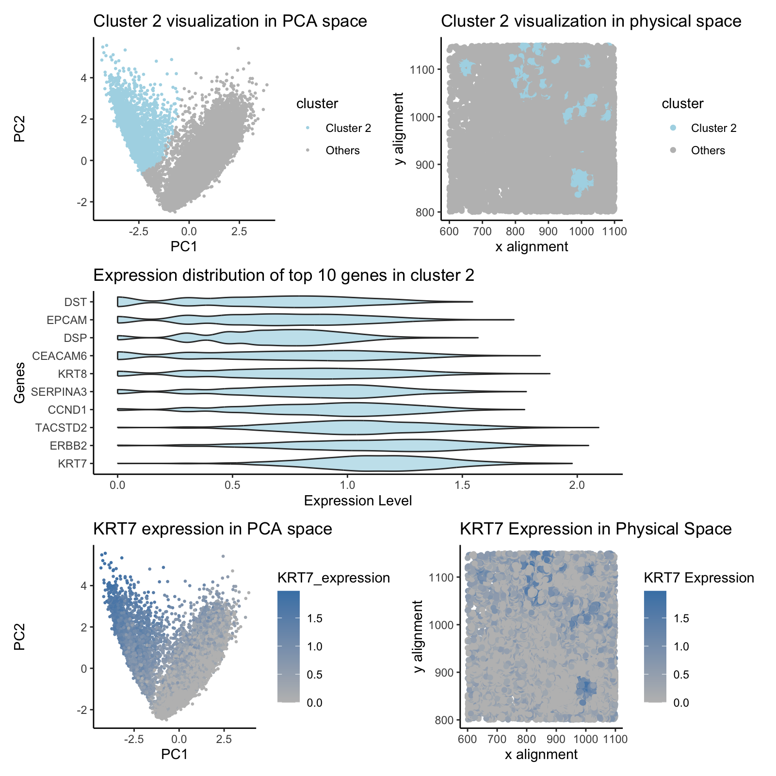
The modification from the HW3 using eevee data set is that I changed the selection of cluster based on the overall cluster visualization in physical space. Method-wise, eevee dataset required heavier quality control over pikachu dataset as the dataset contains lot more data and thus needed to handle some dropouts. The differential gene expression analysis was performed differently to show the top 10 most differentially expressed genes to easily understand the most meaningful DEG analysis. Differentially expressed genes were different from ones from eevee dataset. This figure provides a visualization of Cluster 2, identified through PCA-based clustering of gene expression data. Panel 1 shows the distribution of Cluster 2 in PCA space, demonstrating that it forms a distinct group compared to other clusters. Panel 2 maps the spatial organization of Cluster 2 within the original physical coordinates, reinforcing that cells in this cluster are not randomly distributed but instead maintain a specific spatial pattern.
Panel 3 presents a violin plot of the top 10 most highly expressed genes in Cluster 2, providing insights into the gene expression distribution within this cell population. Notably, KRT7, KRT8, and EPCAM exhibit strong differential expression, suggesting an epithelial lineage. Panel 4 and 5 focus on KRT7 expression, mapping its distribution in PCA space and physical space, confirming that it is highly expressed within Cluster 2.
# data import
file <- '~/Desktop/genomic-data-visualization-2025/data/pikachu.csv.gz'
data <- read.csv(file)

# Load required libraries
library(ggplot2)
library(Rtsne)
library(ggrepel)
library(patchwork)
# Extract positions and gene expression data
pos <- data[, 5:6]
rownames(pos) <- data$cell_id
gexp <- data[, 7:ncol(data)]
rownames(gexp) <- data$cell_id
loggexp <- log10(gexp + 1)

# Perform k-means clustering
set.seed(123)  # For reproducibility
k <- 6  # Number of clusters
com <- kmeans(loggexp, centers = k)
clusters <- as.factor(com$cluster)
names(clusters) <- rownames(gexp)
head(data)
colnames(data)
pos <- data[, c(5, 6)]
rownames(pos) <- data$cell_id
head(pos)
colnames(pos) <- c("X", "Y")

# Perform PCA for dimensionality reduction
pcs <- prcomp(loggexp)
df <- data.frame(pcs$x, clusters)
pca_data <- pcs$x[, 1:20]

ggplot(data) +
  geom_point(aes(x = aligned_x, y = aligned_y, col = clusters)) +
  ggtitle ("Clusters in Physical space") +
  theme(plot.title = element_text(hjust=0.5)) +
  xlab("x alignment") + ylab("y alignment")

# Cluster of interest definition
interest <- 2
cellsOfInterest <- names(clusters)[clusters == interest]
otherCells <- names(clusters)[clusters != interest]
cluster <- ifelse(clusters == interest, "Cluster 2","Others")

# Panel1: Cluster 2 in PCA space
df_pca <- data.frame(pcs$x)
p1 <- ggplot(df_pca, aes(x = PC1, y = PC2, col = cluster)) +
  geom_point(size = 0.5) +
  theme_classic() +
  scale_color_manual(values = c("Cluster 2"="lightblue", "Others"="gray")) +
  ggtitle("Cluster 2 visualization in PCA space")

# Panel 2: cluster 2 in Physical Space
p2 <- ggplot(data) +
  geom_point(aes(x=aligned_x, y=aligned_y,col=cluster)) +
  theme_classic() +
  scale_color_manual(values = c("Cluster 2"="lightblue", "Others"="gray")) +
  ggtitle("Cluster 2 visualization in physical space") +
  xlab("x alignment") + ylab("y alignment")

# Perform differential expression analysis
gexp_cluster_selected <- loggexp[as.numeric(clusters) ==interest, ]  # Expression in selected cluster
gexp_other <- loggexp[as.numeric(clusters) != interest, ]  # Expression in other clusters

pvals <- sapply(1:ncol(loggexp), function(i) {
  wilcox.test(gexp_cluster_selected[, i], gexp_other[, i], exact = FALSE)$p.value
})
adj_pvals <- p.adjust(pvals, method = "bonferroni")

# Compute log fold change
logfc <- colMeans(gexp_cluster_selected) - colMeans(gexp_other)

# Create a dataframe of results
DE_genes <- data.frame(Gene = colnames(loggexp),
                       logFC = logfc, pval = pvals, adj_pval = adj_pvals)

# Filter p-value < 0.05
DE_genes <- DE_genes[DE_genes$adj_pval < 0.05, ]

# Sort by log fold change
DE_genes <- DE_genes[order(DE_genes$logFC, decreasing = TRUE), ]

# Select the top 10 most differentially expressed genes
top10_genes <- DE_genes$Gene[1:10]
print(top10_genes)
# Subset expression data for the top 5 DE genes within the selected cluster
top10_expr <- loggexp[as.numeric(clusters) == interest, top10_genes]

# Extract top 10 most expressed genes in cluster 2
top_genes_cluster2 <- names(sort(colMeans(loggexp[as.numeric(clusters) == 2, ]), decreasing = TRUE))[1:10]

# Create bar plot for top 10 genes in cluster 2?
df_top_genes <- data.frame(gene = top_genes_cluster2,
                           exp = colMeans(loggexp[as.numeric(clusters) == 2, top_genes_cluster2])


# Create violin plot for top 10 genes in cluster 2
library(reshape2)
gexp_cluster2 <- loggexp[as.numeric(clusters) == 2, top_genes_cluster2]
df_violin <- melt(as.data.frame(gexp_cluster2), variable.name = "Gene", value.name = "Expression")
df_violin$Cell <- rep(rownames(gexp_cluster2), ncol(gexp_cluster2))  # Add cell IDs if needed
colnames(df_violin) <- c("Gene", "Expression", "Cell")  # Ensure correct column order


p3 <- ggplot(df_violin, aes(x = Gene, y = Expression)) +
  geom_violin(fill = "lightblue", alpha = 0.7) +
  theme_classic() +
  coord_flip() +
  labs(title = "Expression distribution of top 10 genes in cluster 2",
       x = "Genes",
       y = "Expression Level")

# Now extract KRT7 gene
KRT7_expression <- loggexp[, "KRT7"]
data$KRT7_expression <- KRT7_expression

p4 <- ggplot(df_pca, aes(x = PC1, y = PC2, col = KRT7_expression)) +
  geom_point(size = 0.5) +
  theme_classic() +
  scale_color_gradient(high="steelblue", low="gray") +
  ggtitle("KRT7 expression in PCA space")

# Panel 5: KRT7 expression in Physical Space
p5 <- ggplot(data) +
  geom_point(aes(x = aligned_x, y = aligned_y, color = KRT7_expression)) +
  scale_color_gradient(high="steelblue", low="gray") +
  ggtitle("KRT7 Expression in Physical Space") +
  theme_classic()+
  xlab("x alignment") +
  ylab("y alignment") +
  labs(color = "KRT7 Expression")

#patchwork
combined <- (p1 + p2)/p3/ (p4 + p5)
print(combined)